Fast Robots
Prof. Jonathan Jaramillo
January - May 2024
Grade: A+
My full website for can be found at this link. Below are selected portions.
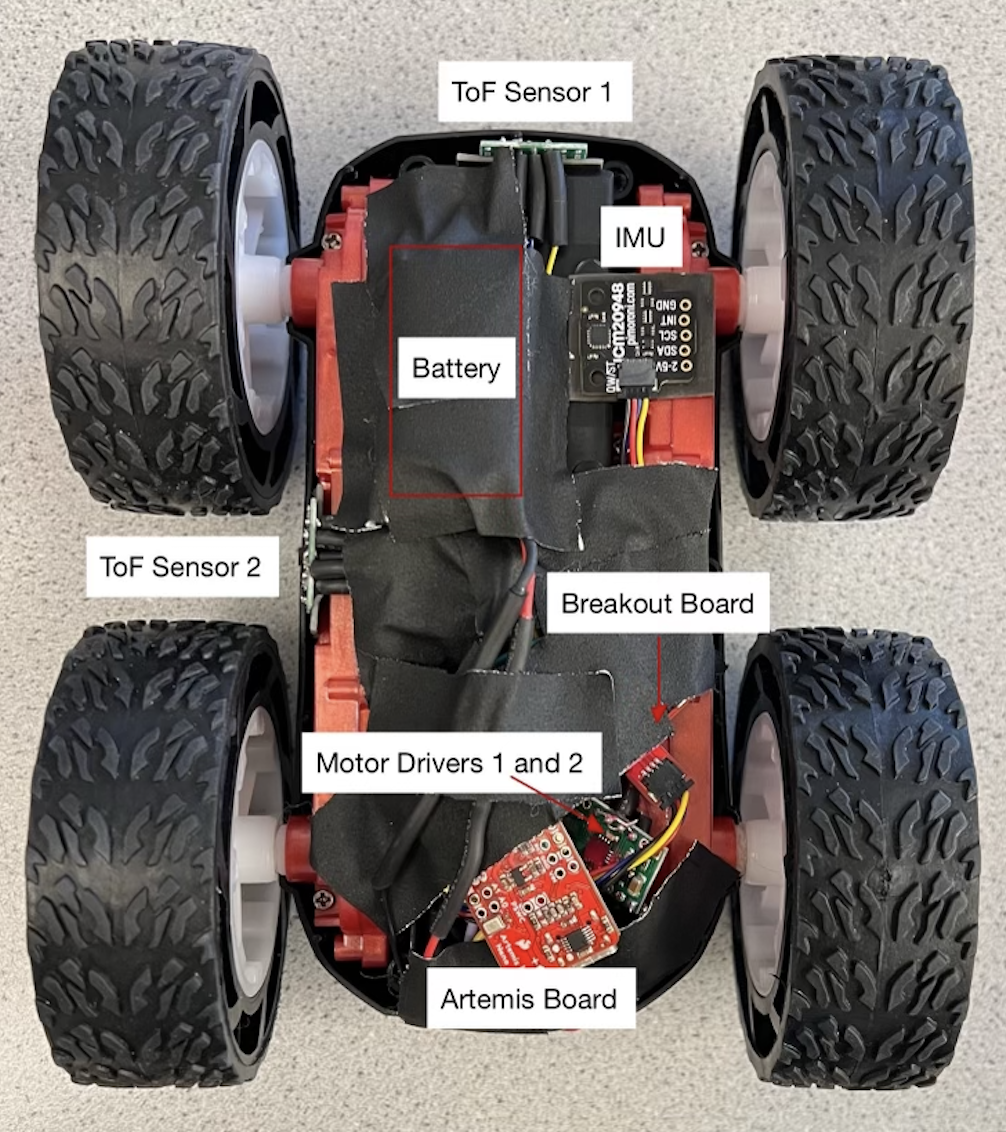
The collective objective of the labs is to collecte IMU and Time of Flight distance sensor data for localization. The below robot was assembled and used throughout the labs.
Objectives
-
Lab 1
- Bluetooth Setup Lab 2
- Reading IMU Data Lab 3
- Time of Flight (ToF) Distance Sensors Lab 4
- Motor Driver Assembly Lab 5
- Linear PID Control Lab 6
- Orientation PID Control Lab 7
- Kalman Filter Using Collected ToF Distance Sensor Data Lab 8
- Implement the Kalman Filter on the Robot Lab 9
- Mapping
- Orientation Control
- ToF Distance Sensor Readings Lab 10
- Localization Simulation
- Write functions to compute the control, odometry motion, prediction step, sensor model, and update step. Lab 11
- Localization on Robot
- Compare the Belief and Ground Truth
- Orientation Control
- ToF Distance Sensor Readings
Lab 11: Localization On The Robot
The objective of the lab is to implement the Bayes Filter on the real robot. Due to noise when the robot is turning, only the update step of the filter will be be used during a 360 degree scan.
Lab Tasks
Simulation Localization
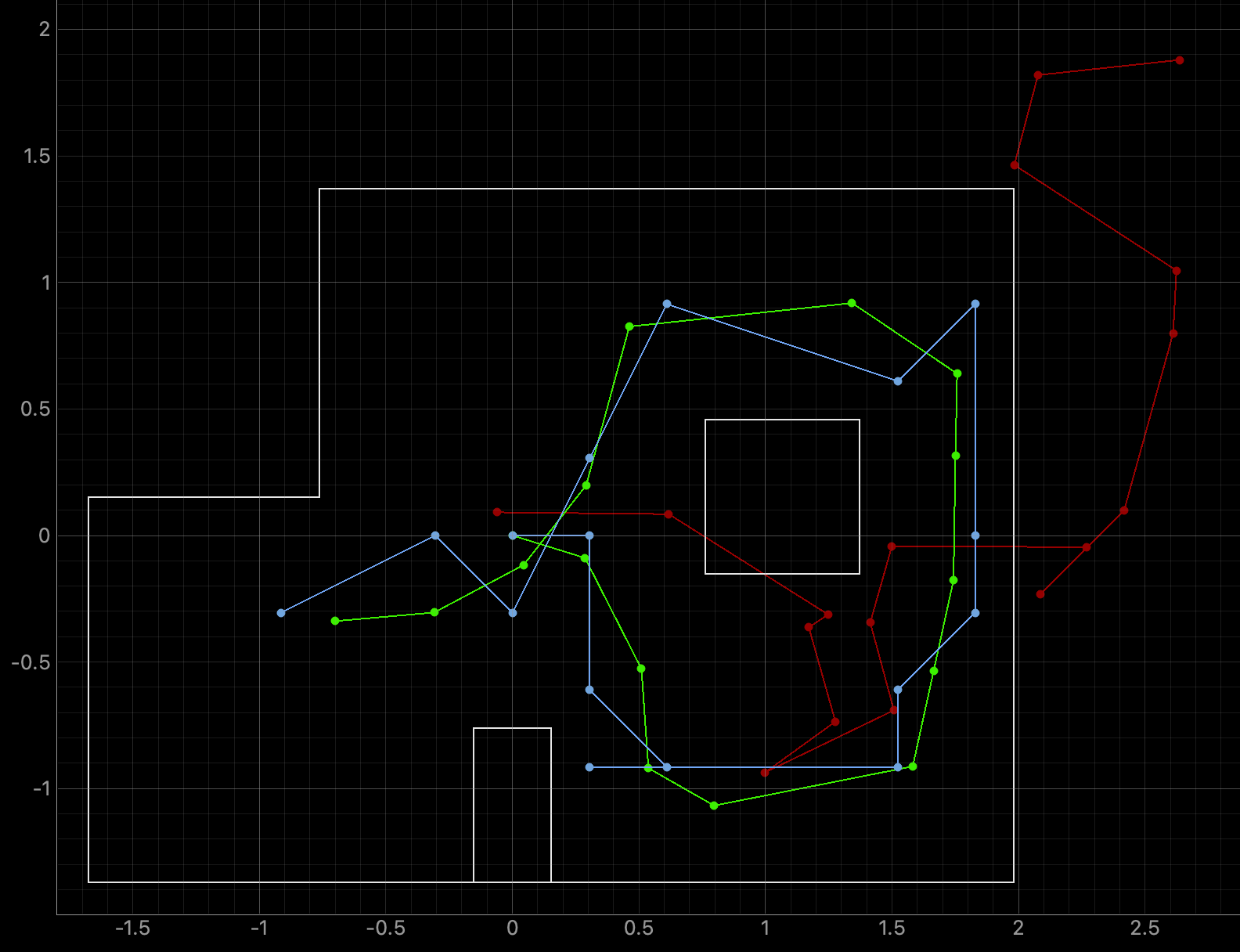
The first lab task was to run the provided Bayes Filter simulation. The lab11_sim.ipynb file was downloaded and a screenshot of the final result is below as well as a link to the data from the simulation. The red line is odometry, the green line is the ground truth, and the blue line is the belief. The map is a three dimensional grid (x, y, theta). The dimension of x is 12, the dimension of y is 9, and the dimension of theta is 18.
Run Robot Localization
The results of rotating the robot at the four marked positions are below. The four marked positions include: (-3ft, -2ft, 0deg), (0ft, 3ft, 0deg), (5ft, -3ft, 0deg), and (5ft, 3ft, 0deg). The robot was run around 4-5 times at each point. Two runs for each point are shown below. The ground truth is plotted as the green dot and is the location where the robot rotated. The belief of the robots position is plotted as the blue dot. The ToF sensor used to collect distance readings was located on the front of the robot, between the left and right sides of the robot. When the robot was at zero degrees the ToF sensor was pointed towards the rightside wall. The robot turned counterclockwise in the same manner as in Lab 9. The Jupyter Notebook code to plot each Ground Truth value is below:
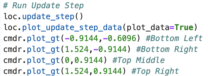
Bottom Left Point (-3ft, -2ft, 0deg):
Graphs for the Belief (blue) and the Ground Truth (green):
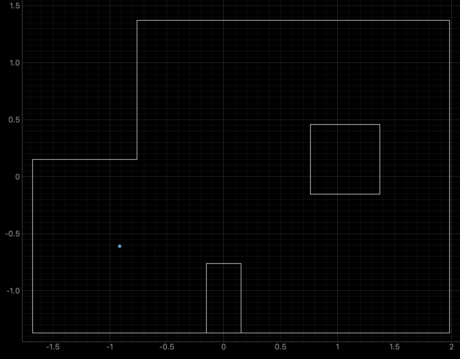
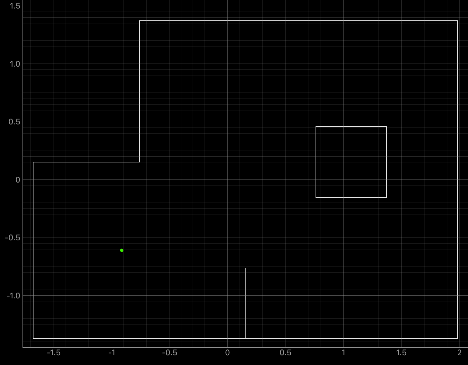
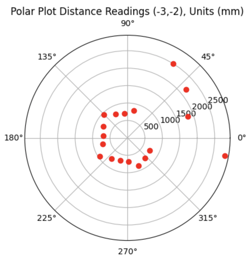
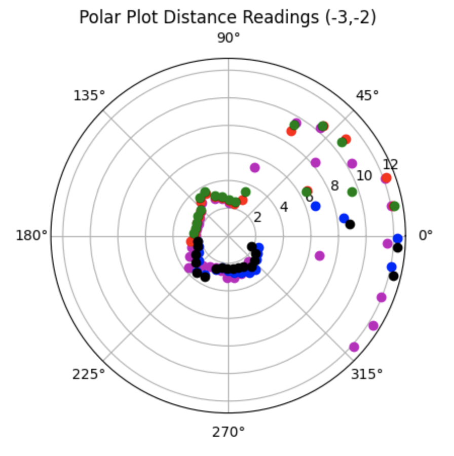
For the bottom left point, the Belief was at the same point as the Ground Truth. As can be seen in the below polar plot, the robot sensed the surrounding walls very well. I reran the rotation several (5) times and this point had the most rotations result in the Belief being the same as the Ground Truth. This is a result of the several walls surrounding the robot when rotating. The next run shows one of the runs where the Belief was different then the Ground Truth.
Polar Plot and recorded data below:
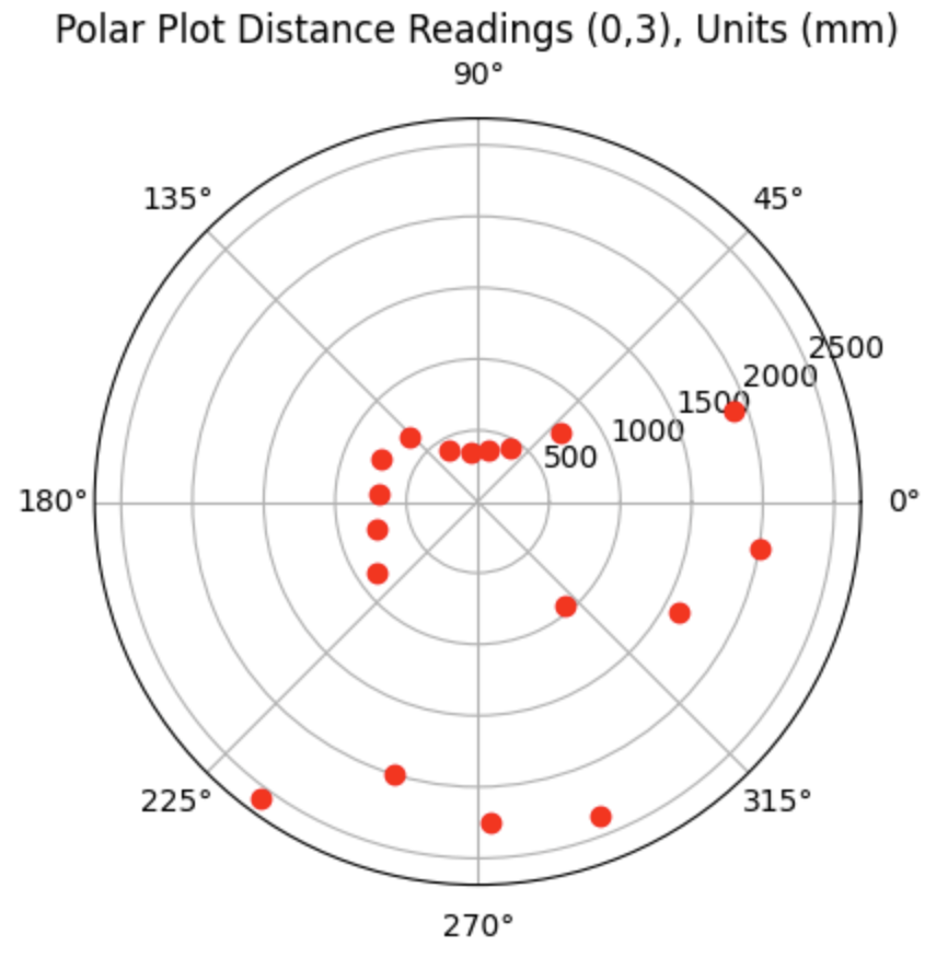
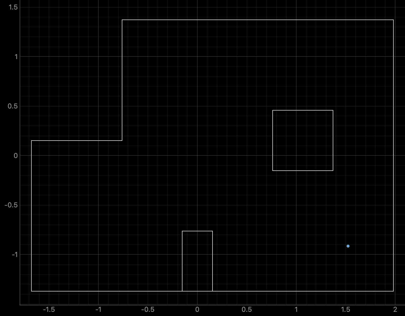
Top Middle Point (0ft, 3ft, 0deg):
Graphs for the Belief (blue) and the Ground Truth (green):
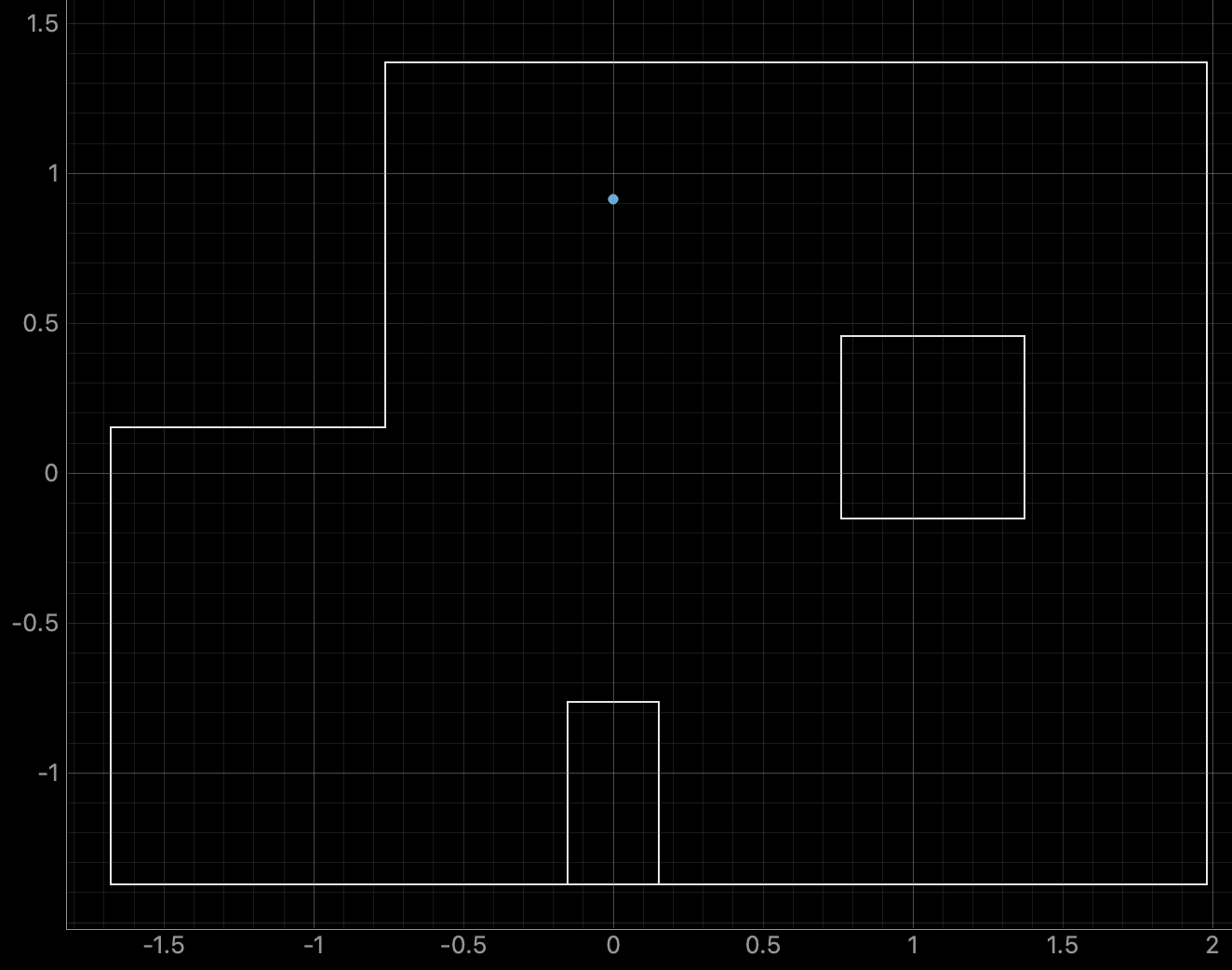
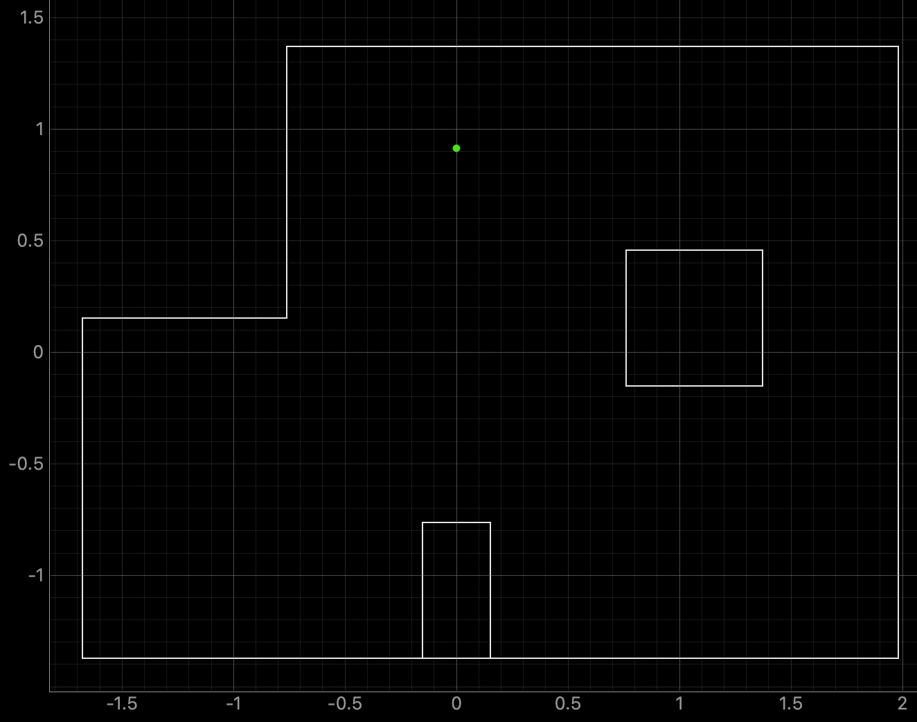
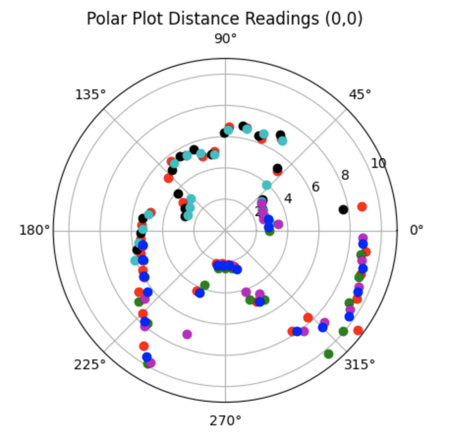
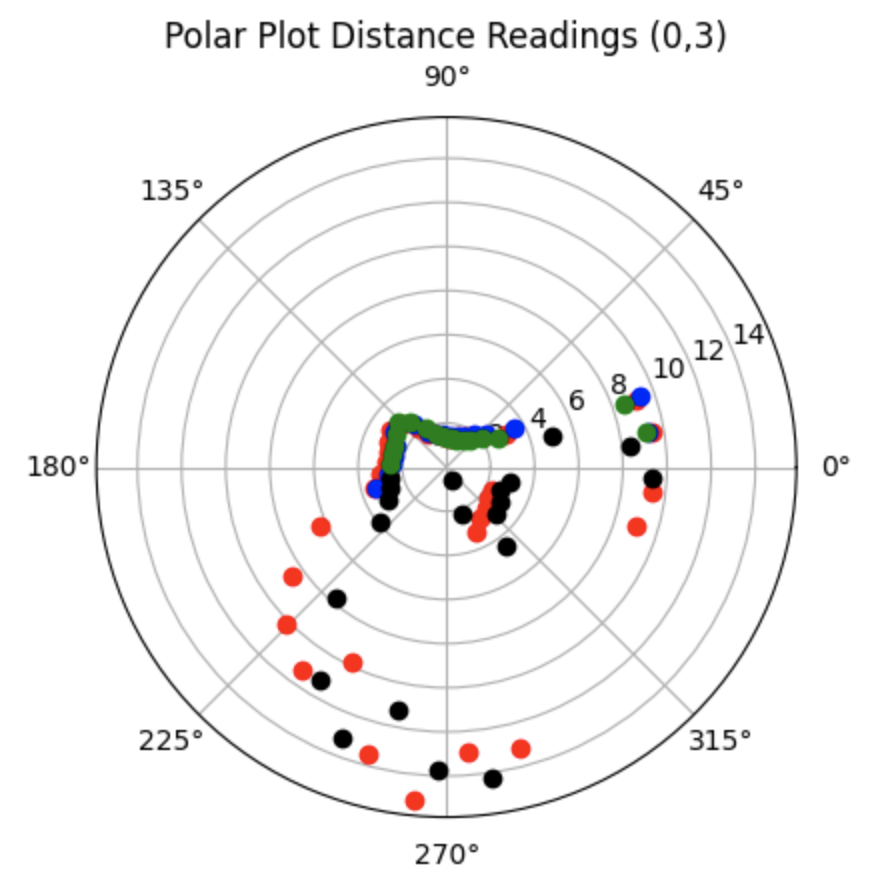
For the top middle point, the Belief was at the same point as the Ground Truth. I was surprised to achieve this result as there are not a lot of nearby walls to use for localization and I suspected that this would be the hardest point to localize. As can be seen in the below polar plot, the robot was able to sense the surrounding walls and obstacles.
Polar Plot and recorded data below:
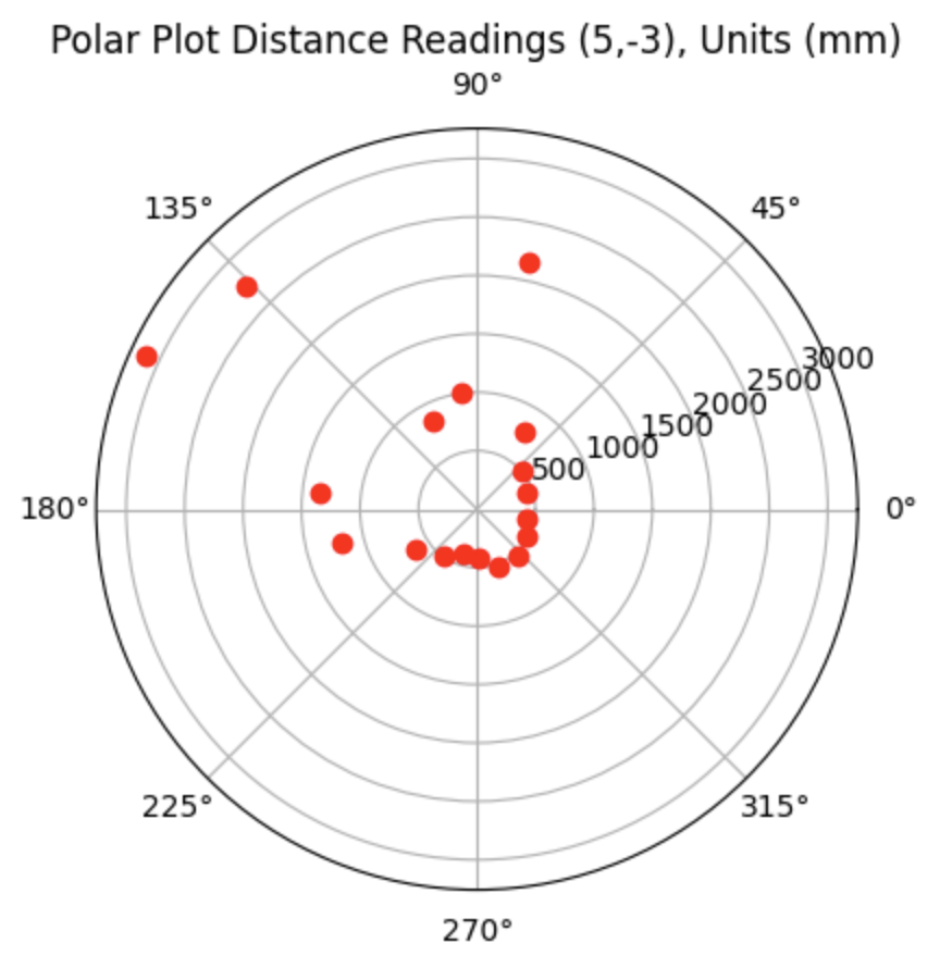
Bottom Right Point (5ft, -3ft, 0deg):
Graphs for the Belief (blue) and the Ground Truth (green):
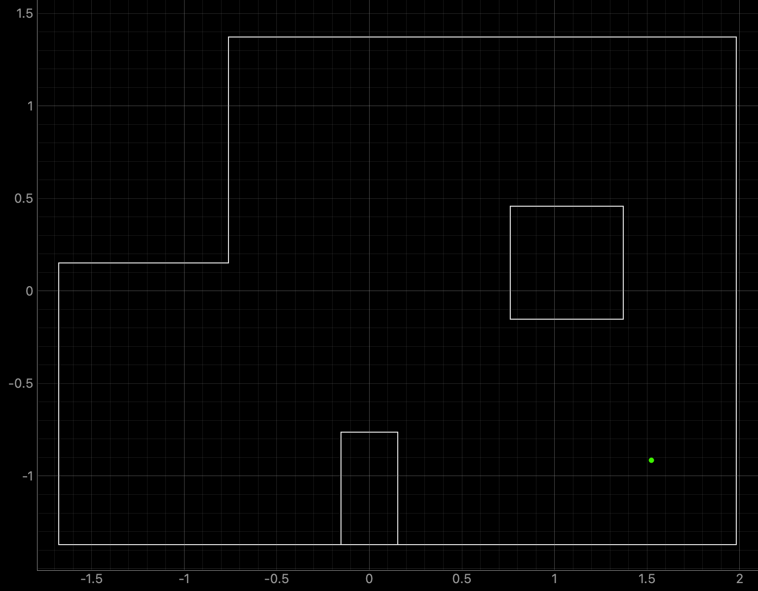
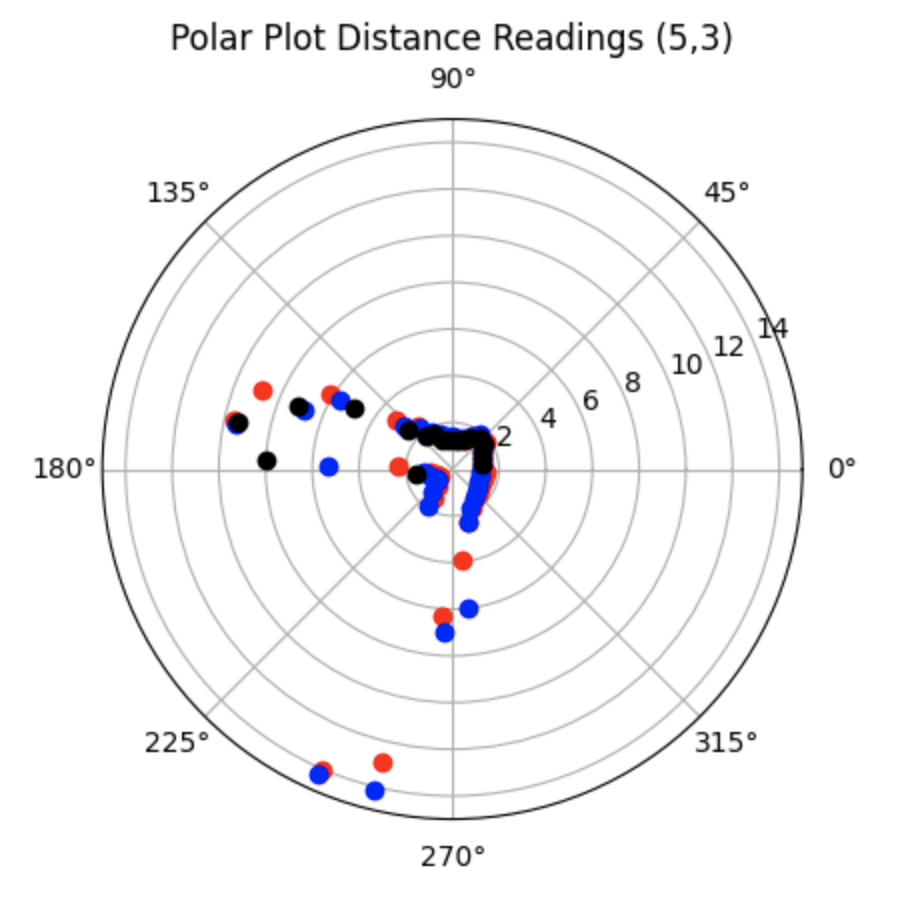
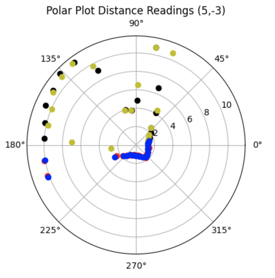
For the bottom right point, the Belief was at the same point as the Ground Truth. As can be seen in the below polar plot, the robot rotated well and was able to sense the surrounding walls and obstacles.
Polar Plot and recorded data below:
Lab 10: Grid Localization Using Bayes Filter
The objective of the lab is to use the Bayes Filter to implement grid localization.
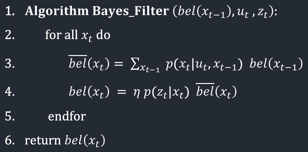
Before starting the lab, I familiarized myself with how the Bayes Filter worked and how to implement the Bayes filter for the robot in simulation. Localization and of the robot determines where the robot is in the enviroment. There is a predition and update step of the Bayes filter. The prediction step uses the control input and accounts for the noise from the actuator to predict the new location of the robot. After the prediction step, the robot rotates 360 degrees gathering distance measurement data. The update step uses the gathered distance measurements to determine the real location of the robot. The Bayes Filter from Lecture 16 is below:
The dimensions of each grid cell in the x, y, and theta axes are 0.3048 meters, 0.3048 meters, and 20 degrees. The grid is (12,9,18) in three dimensions, totalling 1944 cells. The discritized grid map is:
Lab Tasks
Implementation
Five functions were written to run the Bayes Filter as outlined below.
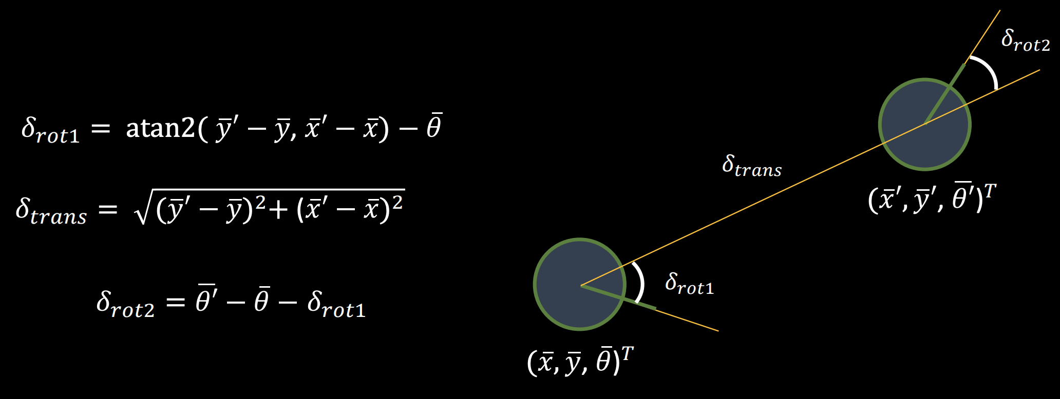
Compute Control
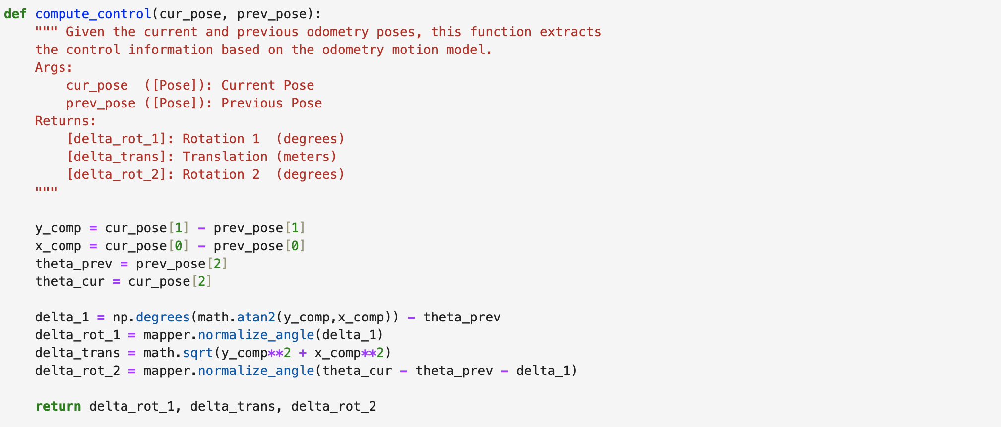
The control information from the robot is used to find the first rotation, translation, and second rotation. The inputs include the current position (cur_pose) and the previous position (prev_pose). The return values include the first rotation (delta_rot_1), the translation (delta_trans), and the second rotation (delta_rot_2). The Lecture 17 slide with the equations to find the odometry model parameters is below:
The above equations were modeled in Jupyter Notebook. The code is found below. First the differences in the y and x positions are found (y_comp and x_comp). Then the normalized rotations are calculated as well as the translation.
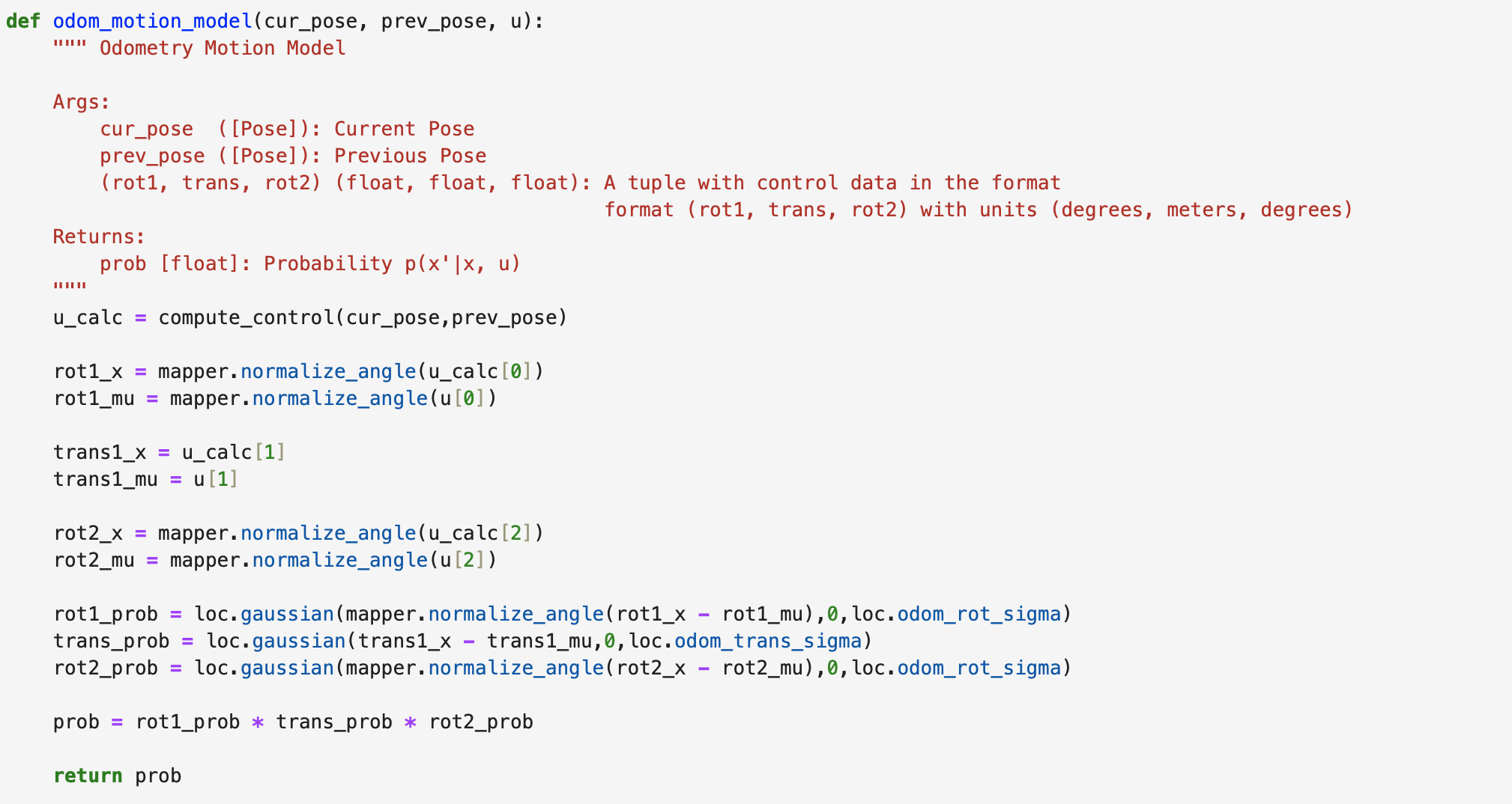
Odometry Motion Model
The odometry motion model finds the probability that the robot performed the motion that was calculated in the previous step. The inputs include the current position (cur_pose), previous position (prev_pose), and odometry control values (u) for rotation 1, translation, and rotation 2. The return value is the probablility ( p(x'|x,u) ) that the robot achieved the current position (x'), knowing the previous position (x) and odometry control values (u). A Gaussian distribution is used. Each motion is assumed to be an independent event. The probability of each event is then multiplied together to find the probability of the entire motion. The Jupyter Notebook code is found below.
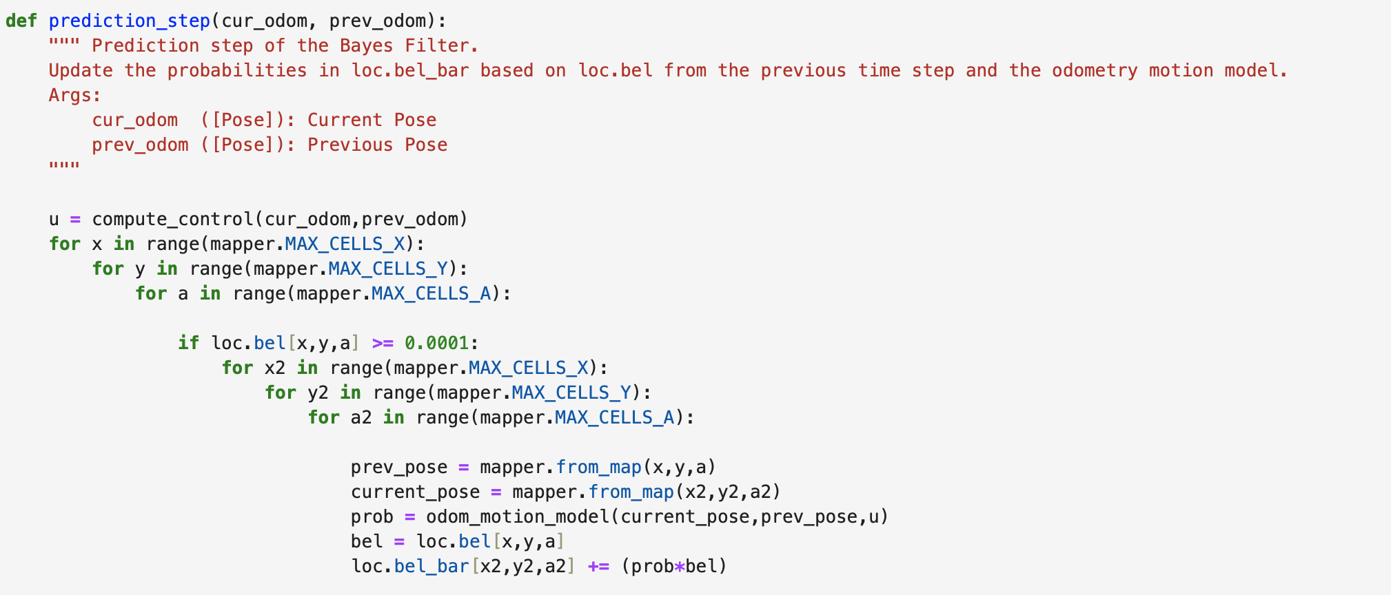
Prediction Step
The prediction step of the Bayes Filter as implemented in Jupyter Notebook uses six for loops to calculate the probability that the robot moved to the next grid cell. The inputs include the current odometry position (cur_odom) and the previous odometry position (prev_odom). The if statement in the pediction step code is used to speed up the filter. If the belief is less than 0.0001 than the three remaining for loops will not be entered as the robot is unlikely to be in the remaining grid cells. If the belief is greater than or equal to 0.0001 the probability will be calculated. The code for calculating the probability is below.
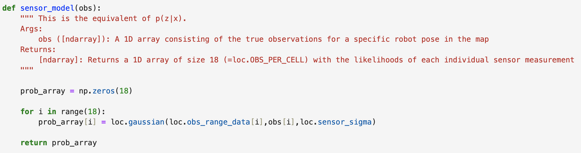
Sensor Model
The sensor model function finds the probability of the sensor measurements, modelled as a Gaussian distribution. The length of the array is 18 as the robot measures 18 different distance reading values. The input includes the 1D observation array (obs) for the robot position. The function returns a 1D array of the same length including the likelihood of each event (prob_array). The Jupyter Notebook code is below.
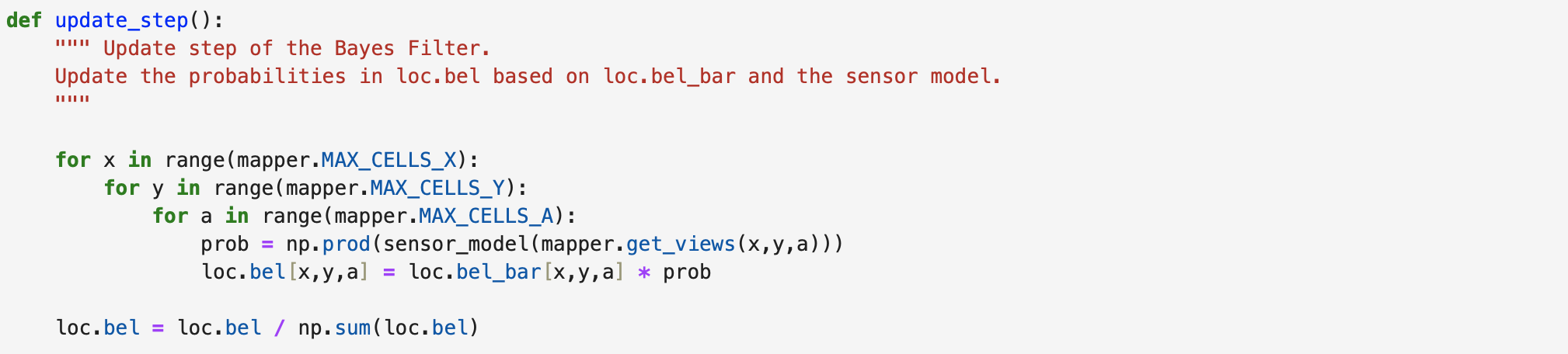
Update Step
The update step calculates the belief of the robot for each grid cell. The probability ( p(z|x) ) is multiplied by the predicted belief (loc.bel_bar) to find the belief (loc.bel). The belief is then normalized. The code can be found below.
Simulation Results
Two runs of the Bayes Filter simulation are found below. The green line is the ground truth, the blue line is the belief, and the red line is the odometry measurements. The lighter grid cells represent a higher belief. For both runs the ground truth and the belief are close together. Both runs were 15 iterations.
Run 1 Results

Run 2 Results

Lab 9: Mapping
The objective of the lab is to use yaw angle measurements from the IMU sensor and distance readings from the ToF sensor to map a room. The map will be used during localization and navigation tasks. Map quality depends on how many readings are obtained and the separation between each reading during each rotation.
Lab Tasks
Orientation Control
Orientation Control was chosen as the PID controller for the lab. The PID controller results in the robot performing on-axis turns in 10 degree increments. The ToF sensor used to collect distance readings is located on the front of the robot between the left and right motor sides.
Code For Orientation Control
First the distance is found using the readings from the ToF sensors, then the yaw angle is found using the IMU sensor. The PID controller value is used in the RIGHT_MOTOR and LEFT_MOTOR functions to determine the motor input value. If the error between the current yaw angle and the setAngle (10 degrees) is less than -0.5 degrees or greater than 0.5 degrees then the RIGHT_MOTOR and LEFT_MOTOR functions will run. The "stop" variable is set to be 360 divided by the "setAngle" variable, which is equal to 10. The results in stop = 36 increments. If variable "end" is less than "stop" the robot will stop for one second. I stopped the robot for one second to ensure that the ToF sensor is pointed towards a fixed point in space. The total yaw angle is recorded by adding the current total to the current yaw value (yaw_arr). The yaw value is then set to zero for the next iteration of the while loop. Resetting the yaw value for the IMU sensor reduces gyroscope drift. If the "end" value is greater than or equal to the "stop" value the robot will stop and no new data will be recorded into the yaw_arr array.
The Jupyter Notebook command and Arduino case to start the PID orientation controller are below. From testing I found that using a Kp value of 1, Ki value of 0 and Kd value of 0 worked to move the robot in 10 degree increments. Each time the PID orientation controller starts, yaw[0], yaw_arr[0], and the total are set to zero. In addition the stop variable is found. Graphs showing the changing yaw angles to confirm the PID controller works are found in the next section.
Video and PID Control Graphs
Two videos of the robot turning are below. The robot roughly turns on axis. In the second video, the robot overshoots at some increments but is able to correct itself to the correct angle. The robot stays inside of one floor tile for the duration of the turn.
Turn 1:
Turn 2:
I plotted the values of yaw for each 10 degree increment. As can be seen in the below graph the PID controller works as expected. After yaw increases to 10 degrees, the value of yaw is reset to zero and then again increases to 10 degrees for the next increment. The slight variation in the final yaw value is due to the -0.5 to 0.5 degree tolerance.
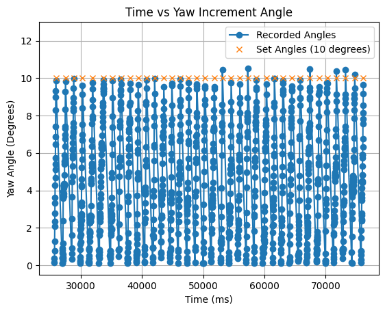
The total angle values were found by adding each final yaw value (between 9.5 and 10.5 degrees) to a summation of all previous yaw values. The values and graph for an example turn are found below.

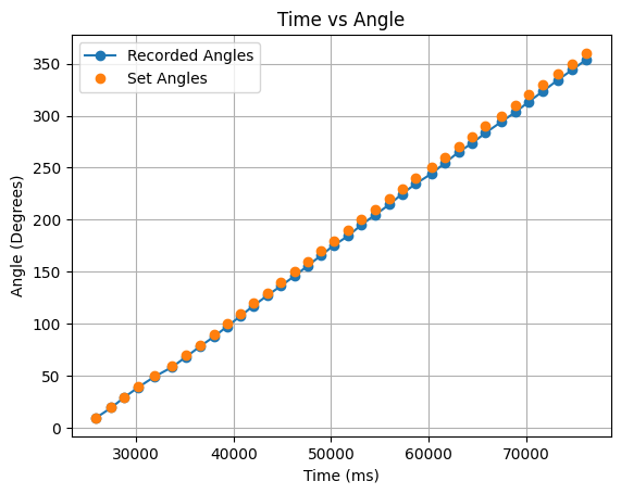
In the above graph as the turn progresses the angles remain accurate as the summation calculation is correct to the yaw reading of the robot, but the angles slightly vary from the ideal 360 degree turn values. To address this I also performed half turns from 0 to 180 degrees, and 180 to 360 degrees. The angle values and corresponding graphs can be found below:


The half turns in the above graphs are more in line with the ideal angles. When testing the robot in the lab, I collected angle data for full turns and half turns.
Read Out Distances
Execute Turn At Each Marked Position
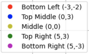
The robot was placed at each of the following points: (-3,-2), (0,0), (0,3), (5,3), and (5,-3). The image below shows each of the points in the lab.

The distance was measured using the front ToF sensor between the left and right motor sides. The data collected was sent over Bluetooth to Jupyter Notebook to be plotted. The robot was started in the same orietation, facing the right side wall of the lab, for each full turn and each half turn starting at zero degrees. For half turns starting at 180 degrees, the robot started facing the left side wall. The range of potential angle values for each ideal 10 degree rotation is 9.5 degrees to 10.5 degrees. There is a -/+ 0.5 degree range for the robot to stop and collect a distance measurement. Due to the range of degree values, it can not be assumed that the robot will stop at exactly 10 degrees every time it rotates. To address this issue, I did not assume that the robot stopped at exactly 10 degrees for every rotation and instead recorded a "total" variable value that added the angle that the robot stopped at to the previously recorded stopping angle. This allowed me to plot the distance measurements with the correct recorded angles.
Polar And Global Frame Plots
This section details the second attempt at collecting data at each point. The data collected for each point in the lab is plotted in the below graphs. I readjusted the ToF sensor to point more upwards before collecting the following data. This adjustement removed noise from inside the map region. The data collected for each point in the lab is plotted in the below graphs.
Bottom Left: Point (-3,-2)
Middle: Point (0,0)
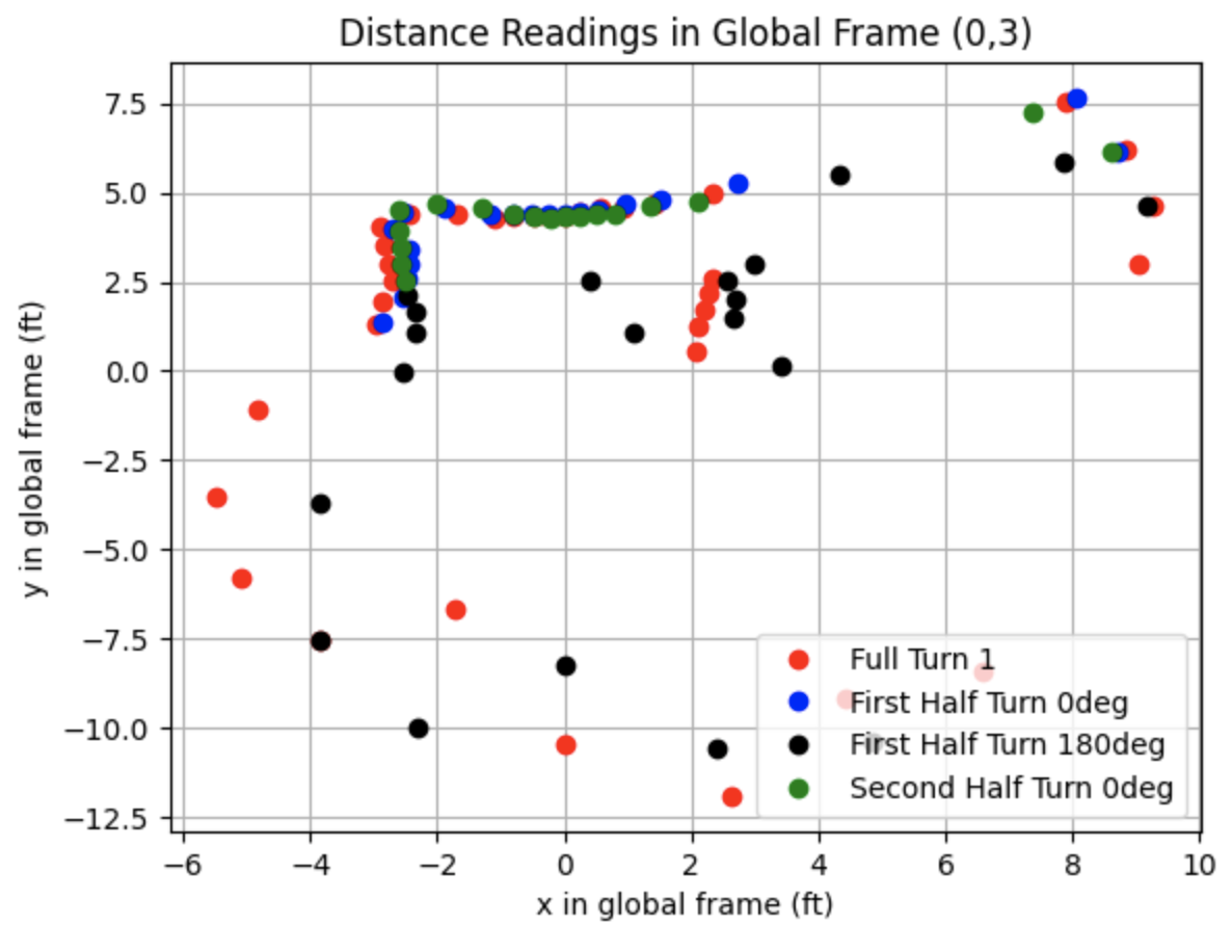
Top Middle: Point (0,3)
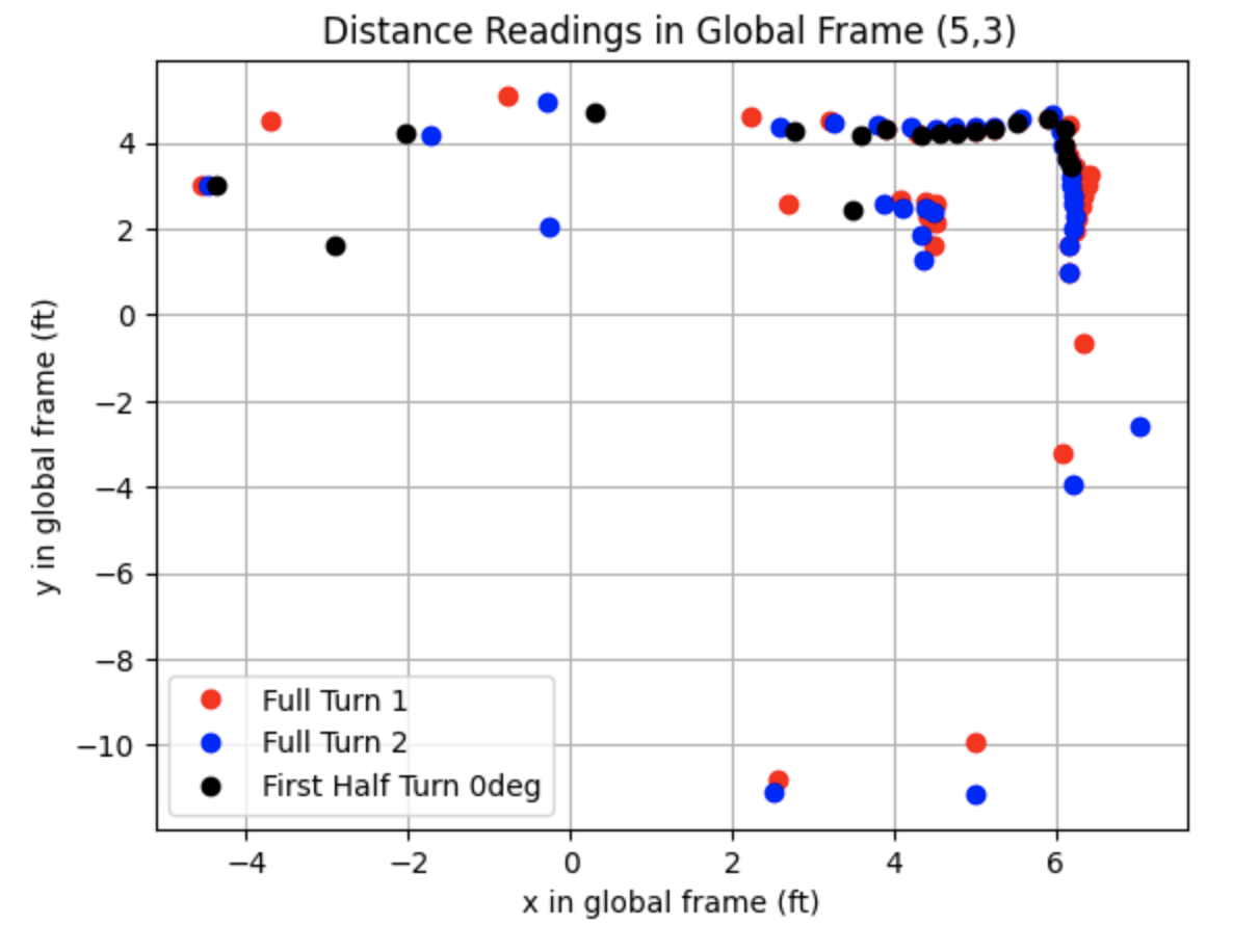
Top Right: Point (5,3)
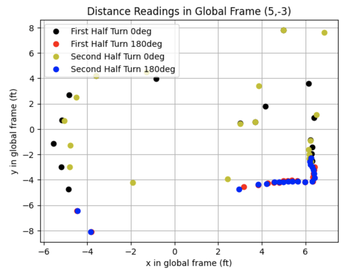
Bottom Right: Point (5,-3)
Merge And Plot Readings
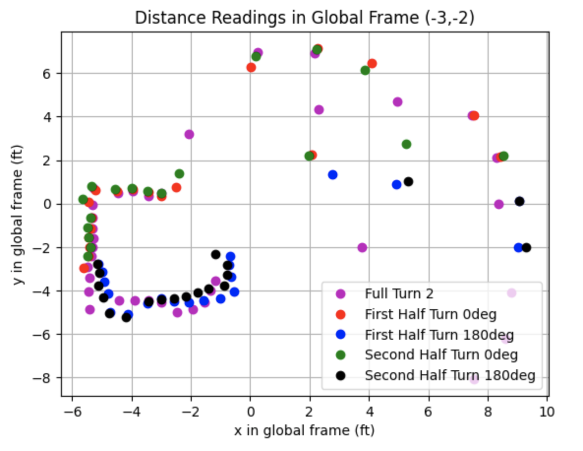
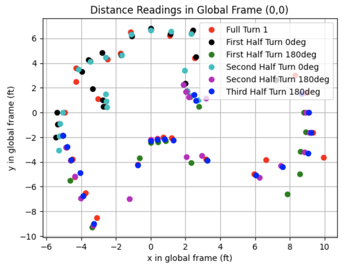
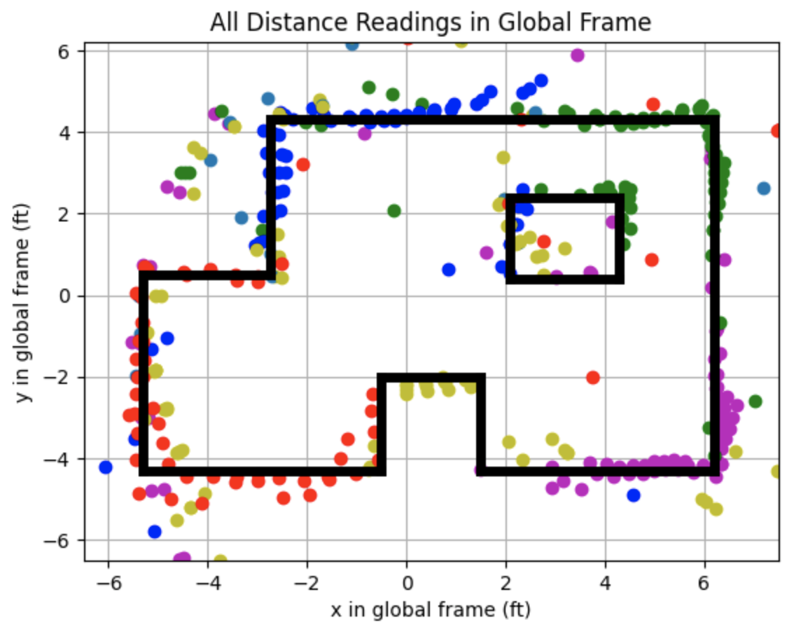
I plotted the distances in the global frame using a transformation matrix to convert the frame of the robot used to collect the sensor measurements into the global frame.
Below are the distance readings in the global frame.
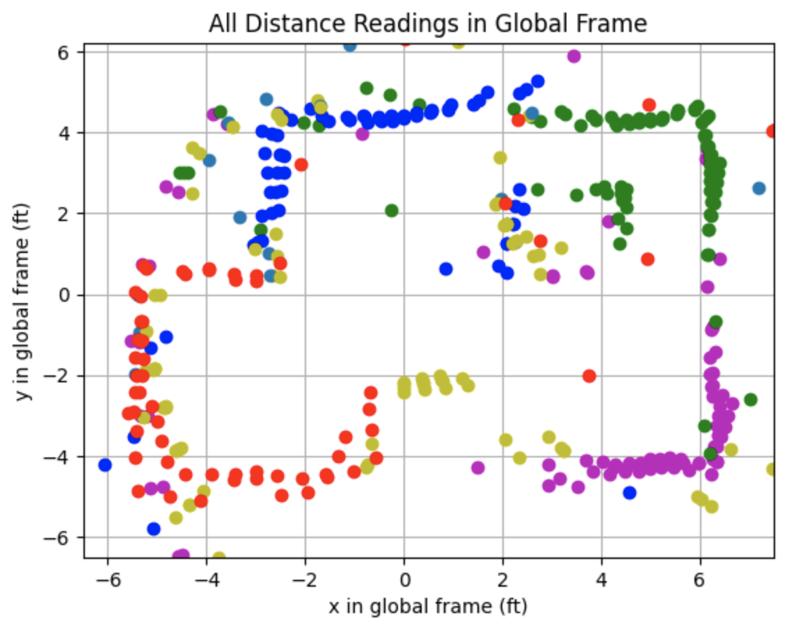
Convert To Line Based Map
After plotting the above graph I plotted lines representing the walls of the map. The plot showing the line based map is below as well as the code used to plot each line.
Lab 8 Extra Credit: Implement Kalman Filter On Robot
I implemented the Kalman Filter on the robot for extra credit. To complete this task I needed to install the Basic Linear Algebra Library on Arduino IDE. To implement the Kalman Filter I first created two new cases in Arduino IDE: KF_DATA and SEND_KF_DATA. These cases are similar to the cases used to start/stop the PID controller and send PID controller data, but I added array's for Kalman Filter time (KF_Time) and the Kalman filter distance (mu_Store). I added a delay in KF_CASE before running the while loop. When I was testing the filter I was repeatedly starting with distances of 0mm. The delay after the ToF distance sensor starts ranging reduces the amount of 0mm distance readings when starting the filter.
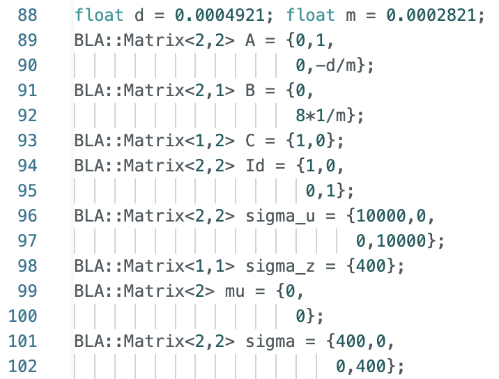
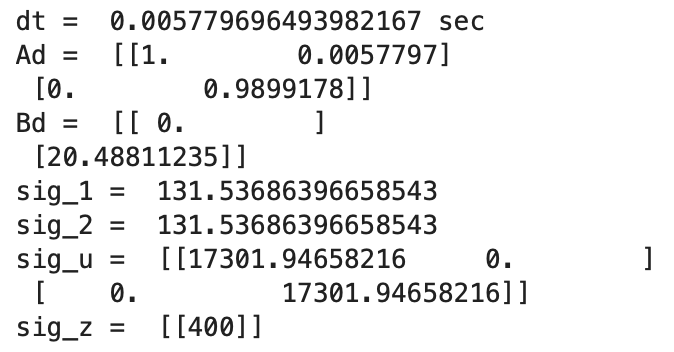
After creating the cases for the Kalman Filter, I then started working on writing a Kalman Filter function in Arduino IDE. The final initialization of the matrices is below:
Step 1: Kalman Filter Function
The first function that I wrote for the lab was the function Kalman_Filter() that is called from inside the larger while loop. To perform this task, I referenced the Jupyter Notebook code I wrote for Lab 7 and modified the code for the Arduino IDE syntax. The function can be seen below:

The Ad (discritized A) and Bd (discritized B) matrices are updated each time the Kalman Filter is called to use the most recent dt value. I printed the dt (time difference) values to the Serial Monitor and observed that the dt values slightly varied each time the while loop ran. The variable dt is how fast the while loop runs and ranged from around 10ms to 25ms. After finding Ad and Bd, mu_p and sigma_p are calculated. The if statement of the filter is the update step and runs when there is a new TOF sensor reading (newTOF == 1). The else statement is the prediction step and assigns the mu_p value to mu and the sigma_p value to sigma. During both steps the first value for mu is stored in the array mu_Store.
Step 2: Kalman Filter Update Step On Robot
Using ToF Readings For PID Loop
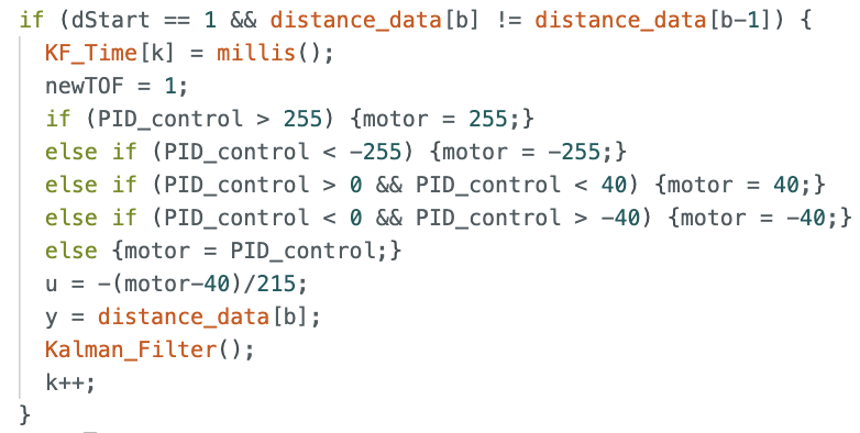
I started working on the calling the Kalman Filter from inside the while loop by modifying the script for my PID controller. After finding the ToF sensor readings and running the PID controller within the larger while loop, I added an if statement inside the loop to call the Kalman Filter to find the update values. The if statement runs if dStart == 1 and if the currect distance value is not equal to the previous distance value. The variable dStart is set to 1 if the new ToF sensor distance is not the same value as the previous sensor distance. If the current distance reading is the same as the previous distance reading dStart is set to 0. The if statement to call the update of the Kalman Filter is below:
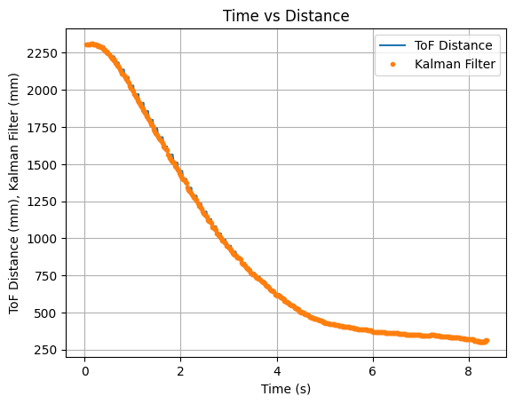
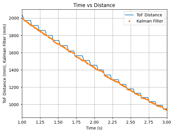
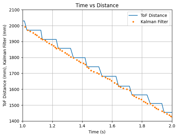
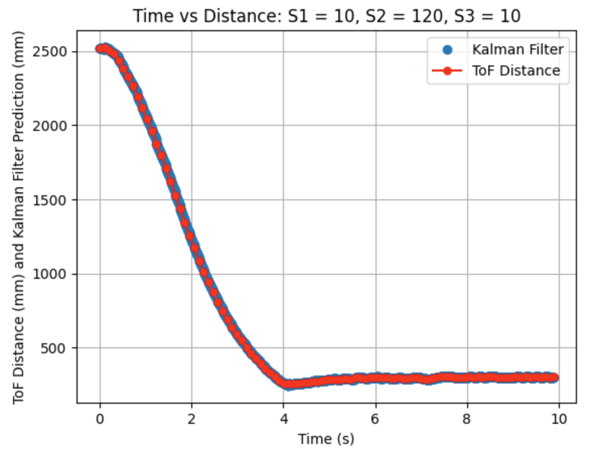
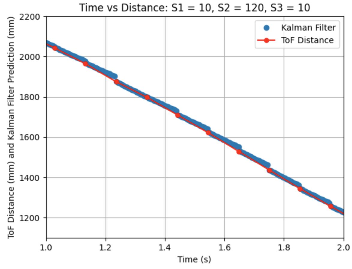
The PID controller was run using values of Kp = 0.05, Ki = 0.0000008, and Kd = 0.5. A test run showing the plotted ToF data and the Kalman Filter updates is shown below. It can be seen that the Kalman Filter updates align with each new reading of the ToF sensor.
The video below shows the Serial Monitor outputs for the ToF distance readings and the update values:
After successfully implemeting the update step of the Kalman Filter, I started working on the prediction step.
Step 3: Kalman Filter Update and Prediction Steps On Robot
Using ToF Readings and Predicted Distances For PID Loop
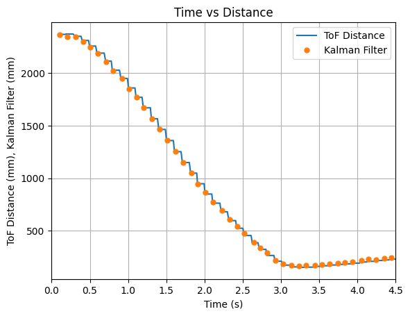
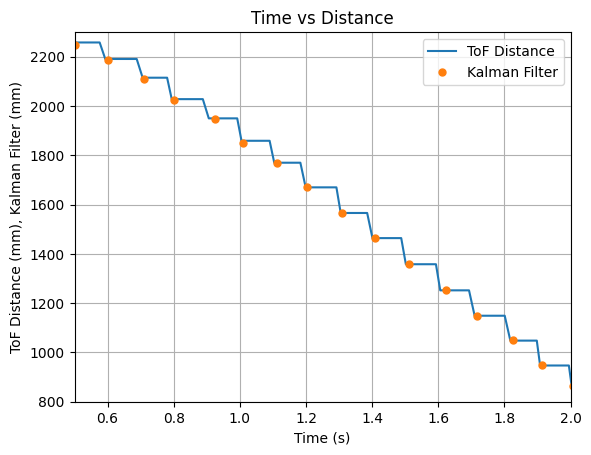
I started the next step by removing the PID control from the larger while loop and creating a separate function called PID_Function(). A separate function for PID control allowed for me to more easily switch the order to performing the Kalman Filter before the PID controller. Previously the PID controller used the ToF sensor measurements every time the loop ran. In the new iteration of the code, if the update step of the filter runs, the distance measurement used will be the ToF sensor reading. If the prediction step runs the most current value of mu will be used in the PID controller. The if and else statements for the update and prediction steps are shown below. The variable dis is the distance measurement used in the PID controller. The u value for the Kalman Filter was calculated the same as in Jupyter Notebook using the PID control values.
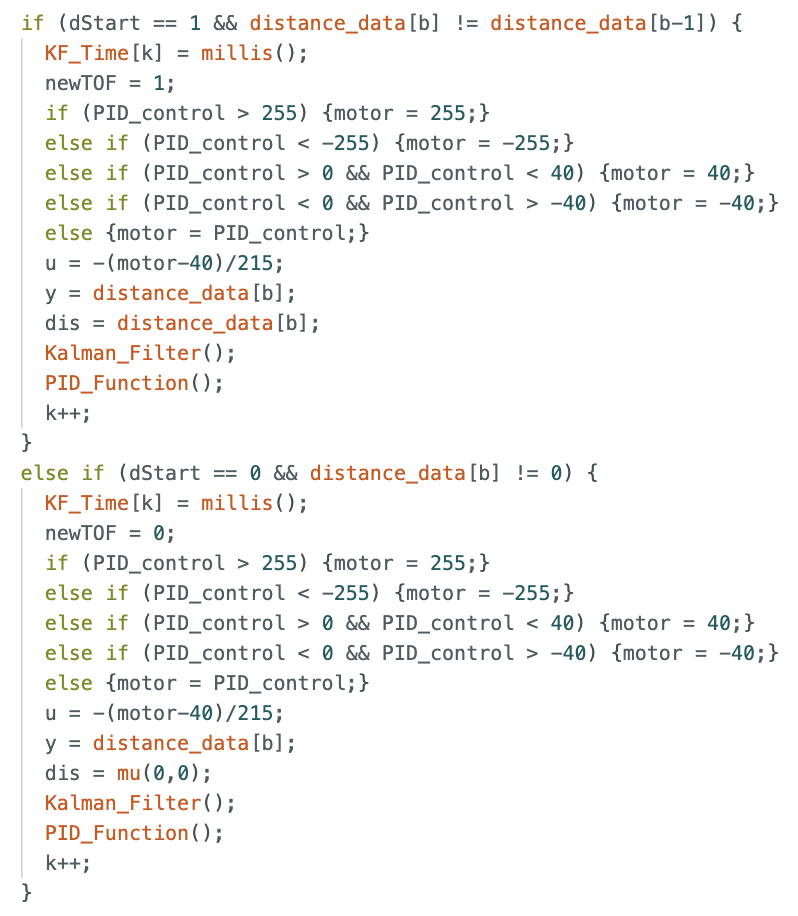
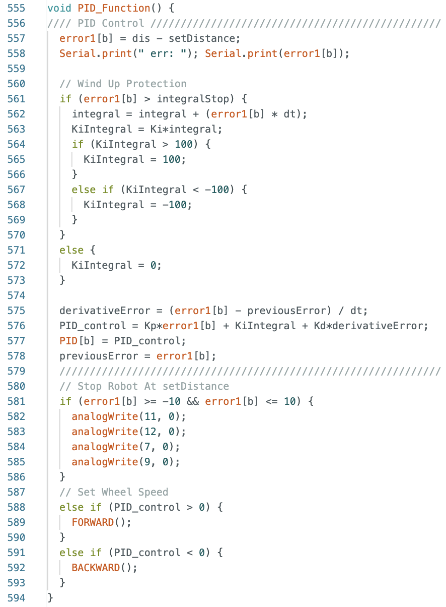
The PID_Function is below:
Throughout testing, I determined that a good value to multuiply the B matrix with is 8. The Kalman Filter updates align with each new reading of the ToF sensor and the prediction values follow the trend of the data. Below are two sets of graphs showing data that was recorded after the B matrix was multiplied by 8. Needing to multiply the B matrix by 8 indicates that the value found for m during the Jupyter Lab simulation does not work as well when implementing the Kalman Filter on the robot.
The video below shows the Serial Monitor outputs for the ToF distance readings and the update values:
Lab 7: Kalman Filter
The objective of the lab is to gain experience implementing Kalman Filters. Labs 5-8 detail PID, sensor fusion, and stunts. This lab is focused on using a Kalman Filter to predict ToF sensor distance readings of the robot. The code from Lab 5: Linear PID Control will be used to gather data, having the robot speed towards a wall and stop 1ft in front of the wall. A Kalman Filter will be implemented in Jupyter Notebook using the collected data.
Kalman Filter Explaination
A Kalman Filter uses a state space model to predict the location (distance from the wall) of the robot. The location of the robot is predicted and then updated using the ToF sensor reading. The prediction and update steps from Lecture 13 are below:

The state space model is used to find the A, B, and C matrices. The state space model for the robot from Lecture 13 is below. The model uses drag (d) and momentum (m) to form the A and B matrices. The two states are the location of the robot and the robots velocity.
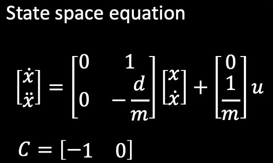
The first part of the lab is estimating the drag and momentum of the robot using steady state velocity. One difference from the lecture slides is that for this lab the C matrix will be C = [1 0]
Lab Tasks
Estimate Drag and Momentum
The drag and momentum for the A and B matrices are estimated using a step response. The robot drives towards a wall at a constant input motor speed. The ToF sensor distance measurements and motor input values are recorded. Velocity is calculated and plotted along with the 90% rise time. The data is used to determine the drag and momentum and build the state space model of the system.
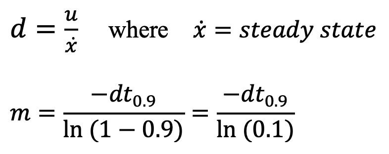
The equations for drag and momentum are below:
The step response u(t) was chosen to be a PWM value of 165. The step response is 64.71% of the maximum u PWM value of 255. I choose a PWM value of 165 as it was the fastest the robot could move while still moving straight for a distance of around 6.5ft. I collected time, ToF distance readings, and used these readings to calculated the velocity. To ensure that the step time was long enough for the robot to reach steady state, I ran the test multiple times.
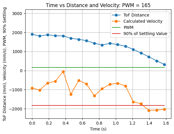
From the above graph it can be seen that the steady state velocity is just over -2000mm/s, or more specifically -2031.91mm/s. Using a 90% rise time a line on the above graph was plotted showing 90% of the settling value. This value is (-2031.91mm/s * 0.9) = -1828.72mm/s. The 90% rise time can be determined from the graph as 1.32s. The steady state velocity is used to find the drag. The drag and rise time are used to find the momentum. The calculations to find drag (d) and momentum (m) are found below:
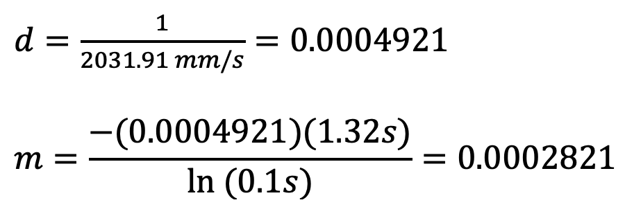
Calculated: d = 0.0004921 and m = 0.0002821
Drag is inversly proportional to the speed of the robot and affects how much the system reacts to changes in u. Momentum relates to how much effort is needed to change the velocity. Higher momentum signifies that more effort needs to be exerted to change the velocity, whereas lower momentum signifies that less effort needs to be exerted to change the velocity.
The collected data array's from all trials were stored in Jupyter Notebook in case the data needed to be used in the future. The code to find the steady state velocity can be found here: Max Speed Code
Initialize Kalman Filter: Python
Compute the A and B Matrices
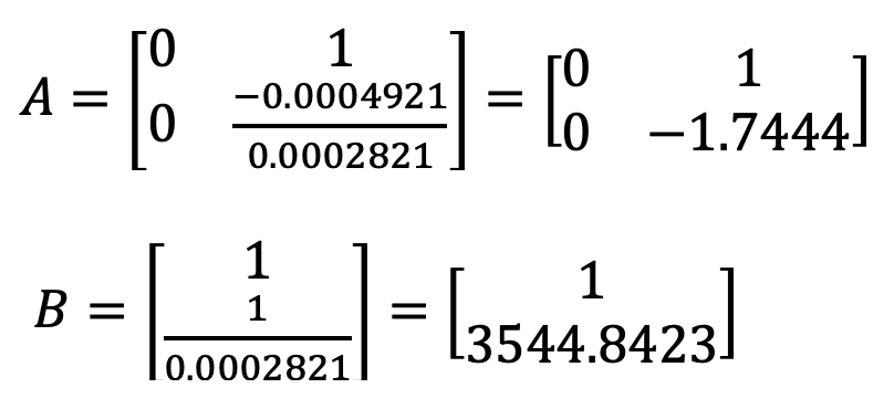
The A and B matrices were computed using the calculated values for d and m. From the state space equation the A and B matrices are:
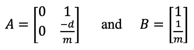
The A and B matrices were calculated as seen below:
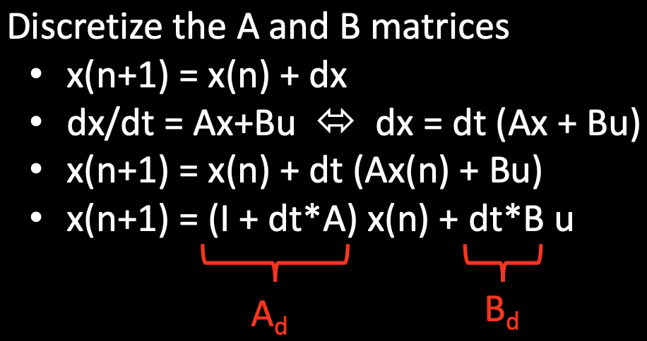
The discritized A and B matrices are calculated using the following method from Lecture 13:
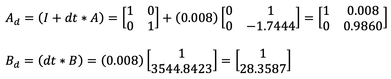
Initially, the sampling time for the discritized Ad and Bd matrices was calculated by subtracting the first time stamp from the second time stamp. After looking closely at the data, the sampling time between each time step was slightly different. I changed the calculation for Delta_T to be an average of all of the sampling time differences. The Delta_T was recalculated for each new dataset that I graphed. Below is an example calculation of the discritized Ad and Bd matrices, using the found sampling time of 0.008s for the PID loop in Lab 5. This dt is how fast the PID control loop is running.
The provided code in the lab report as well as my method of finding Delta_T was used to implement the calculation in Python as seen below:
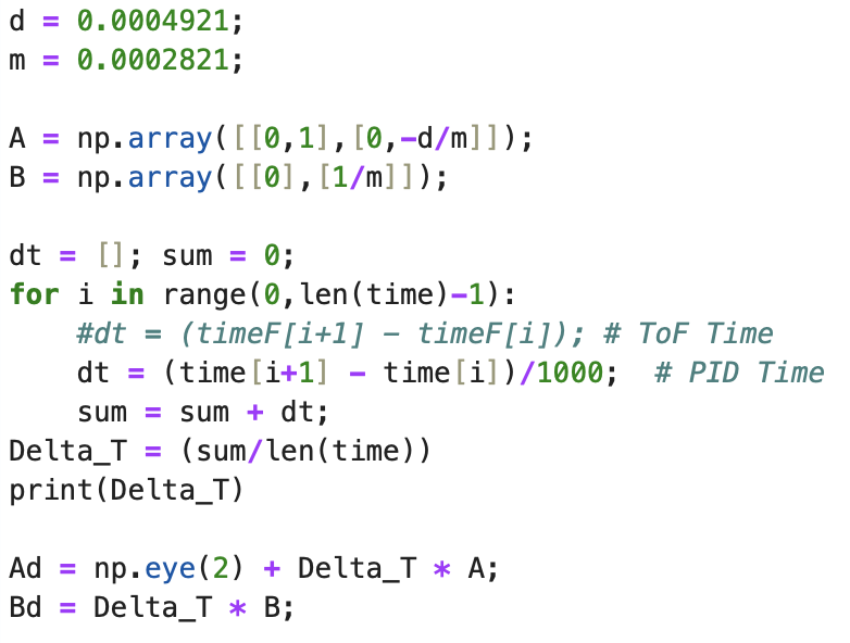
There are two different time array's. One method of finding Delta_T uses the time array of the PID controller (array: time). This method was for the 5000 level task, resulting in a faster frequecy than the frequency found for the ToF readings (array: timeF). In between ToF readings the prediction step of the Kalman Filter estimates the state of the robot.
The previously used code that does not calculate the average sampling time to find Ad and Bd can be found here: Previous Ad Bd Code
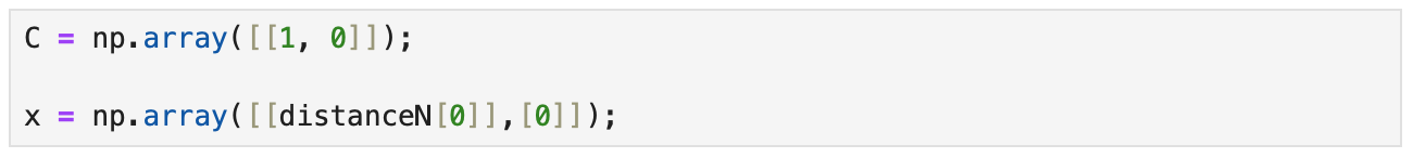
Identify the C Matrix and Initialize the State Vector
The C matrix for the state space is C = [1 0]. C is an m x n matrix where m is the number of states measured (1, ToF sensor distance) and n is the dimensions of the state space (2, ToF distance and velocity). The initial state is the first distance measurement and a velocity of 0 as the robot is not yet moving. The positive distance from the wall was measured.
Below is the Python code to establish the C matrix and initialize the state vector for the ToF distance measurements.
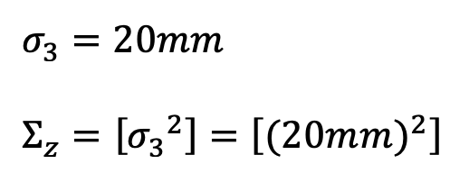
Specify Process Noise and Covariance Matrices
The process noise and the sensor noise covariance matrices need to be specified for the Kalman Filter to work well. Sigma_3 was initialized as 20. This value was determined from slide 35 in Lecture 13 as well as the ToF sensor datasheet. Sigma_Z represents the mistrust in the sensor readings. The ToF sensor has a ranging error of +/- 20mm in ambient and dark lighting.
Sigma_1 and sigma_2 were initialized using the calculation found on slide 35 of Lecture 13. Sigma_U represents the mistrust in the Kalman Filter model. Sigma_1 is the relationship between the ToF distance reading and the model predictions. Sigma_2 is the relationship between the velocity and the model predictions.
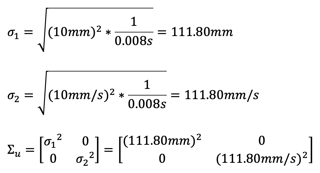
In Jupyter Notebook, I calculated the sigma values for each dataset as shown in the below code. The initiallized sigma had a value of 20 for sigma_1 and 5 for sigma_2 as the robot is not moving initially.
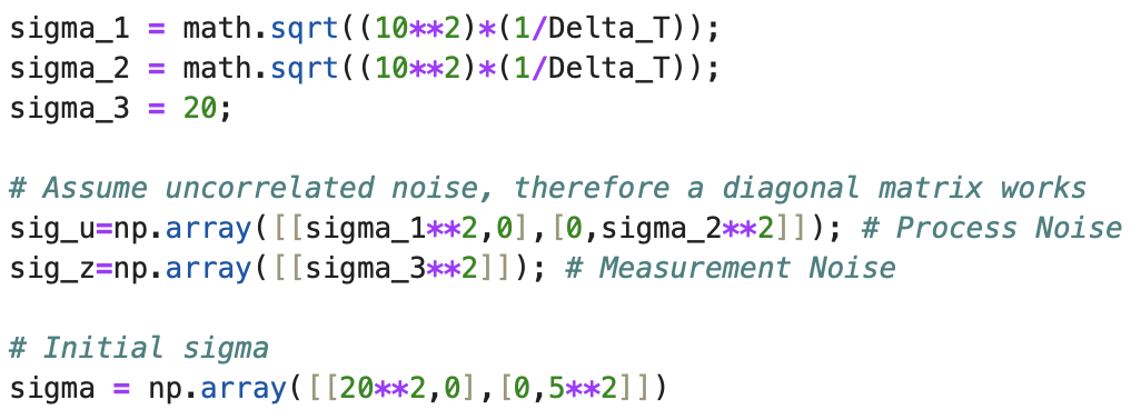
The sigma values were altered as needed for each dataset.
5000 Level Task: Faster Frequency Kalman Filter -- And -- Implement and Test Kalman Filter: Python
The below section includes the 5000 level task to use a faster frequency and use the Kalman Filter prediction step to estimate the state of the car, as well as the same data graphed without the prediction step for comparison. To write the below code I went to office hours to ask questions and looked at all of the lab reports for the TAs.
The below code for the Kalman Filter function was provided in the lab instructions and implemented in Jupyter Notebook.
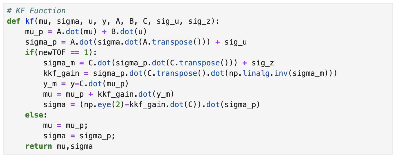
The first two lines finding mu_p and sigma_p are the prediction step of the Kalman Filter. If there is no new ToF sensor reading, then the returned mu and sigma will be equal to what is found during the prediction step. Within the if statement there is the update step of the Kalman Filter that runs every time there is a new ToF reading. The current state is mu, the uncertainty is sigma, the motor input values are u, and the distance readings are y.
To loop through each time step the below code was used.
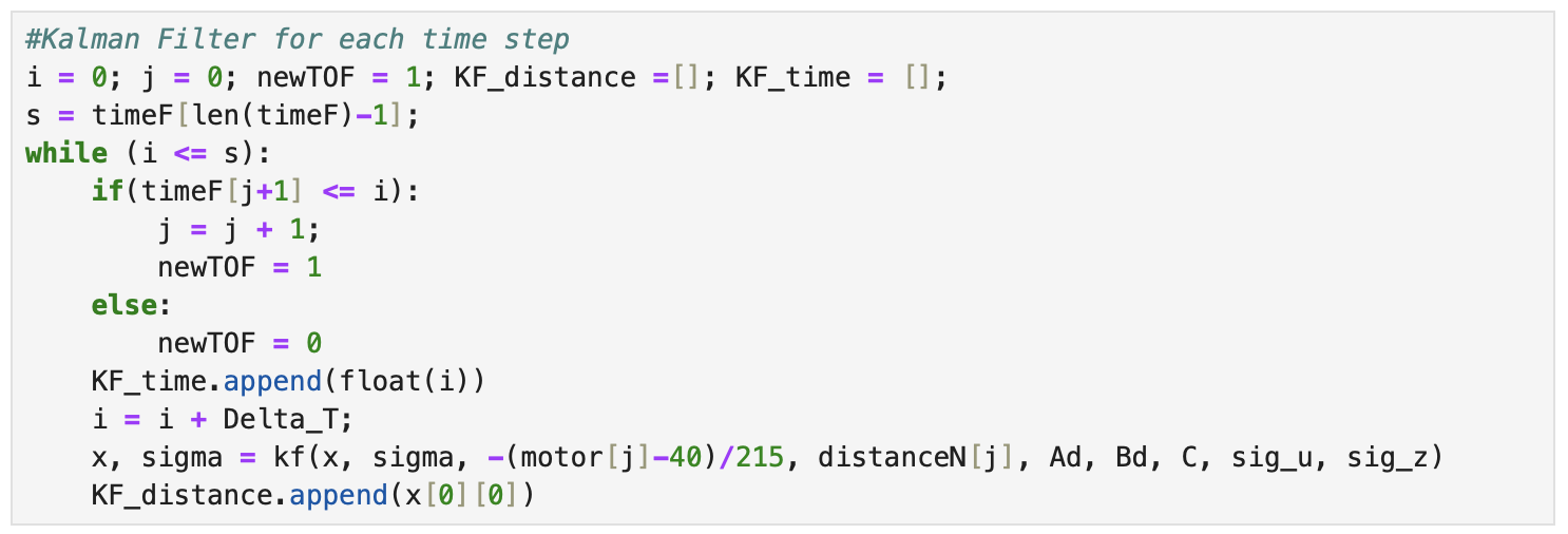
The while loop determines how many times the Kalman Filter runs. How many times the while loop runs depends on the the second to last time step for a ToF sensor reading and the value of Delta_T. If the value of the ToF time array is less than or equal to the value of the index, i, then the value of newTOF will be set to 1 and the update step of the Kalman Filter will run. If the value of the ToF time array is not less than or equal to the value of the index, i, then the value of newTOF will be set to 0 and only the prediction step of the Kalman Filter will run. The index i is updated by adding Delta_T each time the while loop runs and the value of i is appended to the array KF_time to plot the Kalman Filter. After i is updated, the Kalman Filter function is called and then the output distance (x) is appended to the KF_distance array to later be plotted. The u input was the negative value of 40 subtracted from the motor array storing PWM values, divided by 215 (the upper bound of 255 minus the lower limit of 40). The lower limit PWM value is 40. In this model if the motor input value is 40 then the value for u is zero (-(40-40)/215).
Filter Parameters
Throughout the lab report I discuss the parameters used to modify the Kalman Filter and in the section below I discuss how the parameters are modified to better fit the Kalman Filter to the ToF distance data. To summarize, the parameters include the sampling time (Delta_T), drag (d), momentum (m), and sigma values including Sigma_1, Sigma_2, and Sigma_3. The sigma values are used to find the covariance matrices: Sigma_U and Sigma_Z. Sigma_U represents the confidence in the model (distance and velocity) and Sigma_Z represents the confidence in the sensor measurement. Drag is inversely proportional to speed and momentum is related to how much effort is needed to change the speed of the robot. In extension, the values for drag and momentum affect the A and B matrices. Delta_T and the A and B matrices affect the values of the Ad and Bd matrices.
Kp = 0.05, Ki = 0.000008, Kd = 8
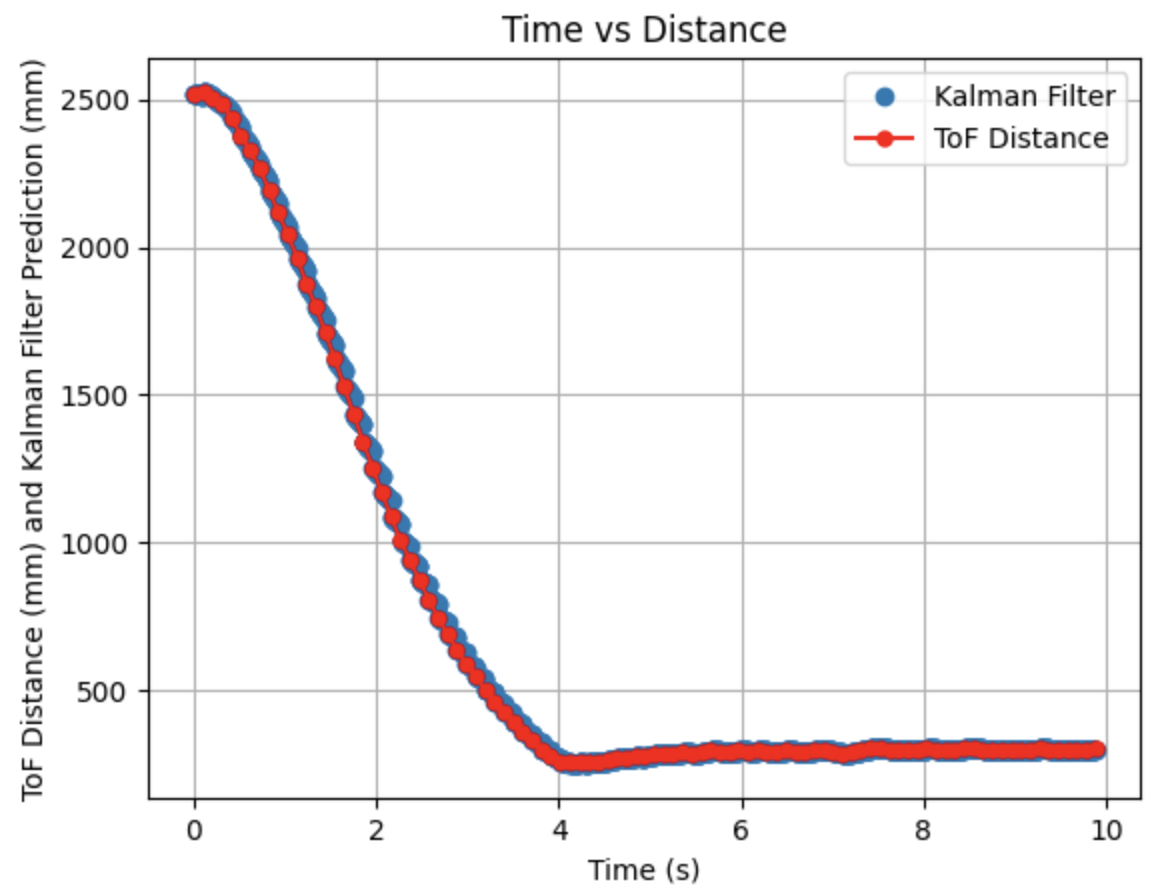
Initially running the Kalman Filter results in the above graphs. The calculated Delta_T for the PID controller is 0.0058 seconds, a frequency of 172.41Hz. The Kalman Filter is running at a faster frequency than the ToF sensors. The maximum PWM value is 115. Sigma_1 and Sigma_2 are 131.54 and Sigma_3 is 20. Overall, the model works well, but the predictions could be more inline with the ToF distances. In the next step I modify the parameters to adjust the prediction values.


I adjusted the parameters for Sigma_1, Sigma_2, and Sigma_3. Decreasing Sigma_1 to 10 (model uncertainty for location) and Sigma_2 to 120 (model uncertainty for velocity) indicates that the model is more accurate than what was initially predicted. Sigma_3 (sensor uncertainty) was changed to 10 as the sensor readings were reliable. All other parameters (d, m, and Delta_T) were kept the same as the previous step. As can be seen from the graphs the Kalman Filter more closely follows the trend of the distance measurements.

In the above graph I kept all previously found parameters the same but changed the value of the increment "i" in the while loop in the same manner as I did for Graph 1. The line changed from "i = i + Delta_T" to "i = i + 2*Delta_T". This change results in less Kalman Filter predictions to be plotted and the same offset behaviour as seen in Graph 1.
Lab 6: Orientation PID Control
The objective of the lab to to gain experience working with PID controllers for orientation. Labs 5-8 detail PID, sensor fusion, and stunts. This lab is focused on using a PID controller for orientation control of the robot. The IMU will be used to control the yaw of the robot.
PID Control Explanation
For this lab a PID controller will be used for orientation control of the robot. The below equation from the course Lecture 7 is used to compute the value for the PID controller:
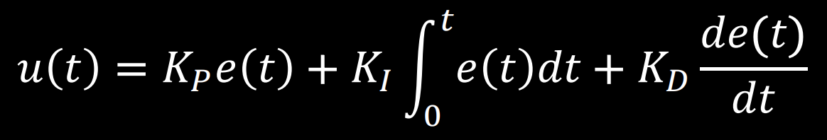
This equation uses the error e(t) (difference between the final desired value and the current value) in proportional, integral, and derivative control to calculate the new PID input value u(t). For this lab the error is the difference between the desired angle (yaw) and the robots current angle (yaw). The calculated PID input value is related to the robots angular speed. Proportional control multiplies a constant Kp by the error. Integral control multiplies a constant Ki by by the integral of the error over time. Derivative control multiplies a constant Kd by the rate of change of the error.
Lab Tasks
PID Input Signal
Integrate Gyroscope To Estimate Orientation
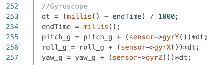
The gyroscope reading was integrated using the following lines of code:
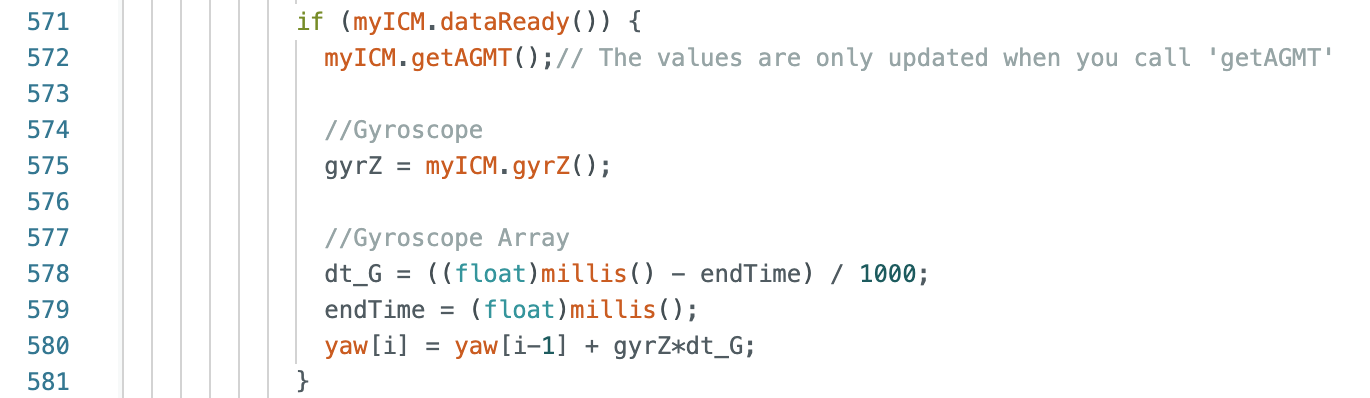
These lines of code are within the larger while loop and each time the while loop runs the gyroscope updates the sensor readings. Yaw is then found using the previous yaw reading, the gyroscope reading, and the calculated difference in time.
Orientation Control
For the orientation control task the robot uses a PID controller and the calculated yaw angle from the gyroscope readings to move towards and maintain the set angle. The implemented PID controller works for various angles and on different floor surfaces.
Rotational Lower Limit PWM
While I was initially testing the PID controller the lower limit PWM value was set to the same as the lower limit value of 40 from the previous lab. Using a lower limit of 40 resulted in the robot getting stuck and not fully turning. I created a new Arduino case and Jupyter Notebook command to find the lower limit PWM for turning. After testing various PWM values, I found that a lower limit value of 120 resulted in the robot turning.
Proportional Control (Kp)
I started with testing the proportional controller. I worked on finding a value for Kp, while keeping Ki and Kd zero. I choose an angle of 180 degrees to start testing the proportional controller. I estimated the Kp constant to be 1.4167 when testing 180 degrees. The equations are found below:
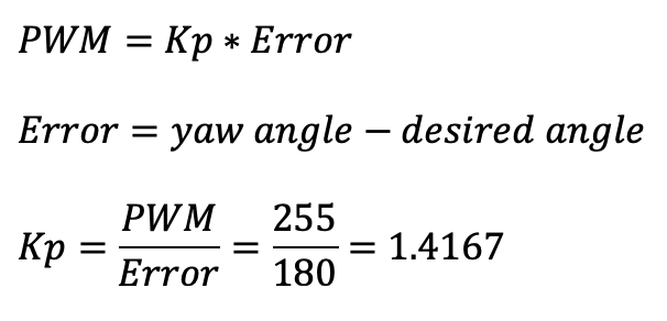
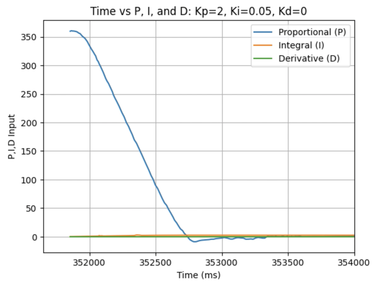
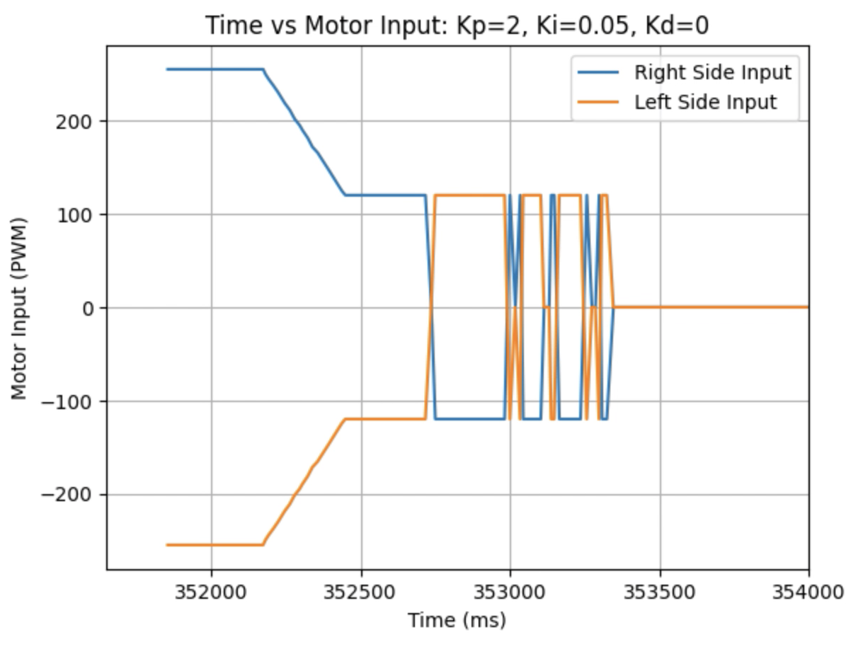
During physical testing I wanted the proportional control to slightly over shoot the desired angle. The over shoot will be addressed using derivative control and the speed will be addressed using integral control. A range of Kp values including 1, 1.5, 1.75, and 2 were tested as can be seen in the below graphs showing yaw, error, PID components, and motor input. I determined that the Kp value should be 2. The code for the proportional controller is below:
Graphs for Kp = 2:
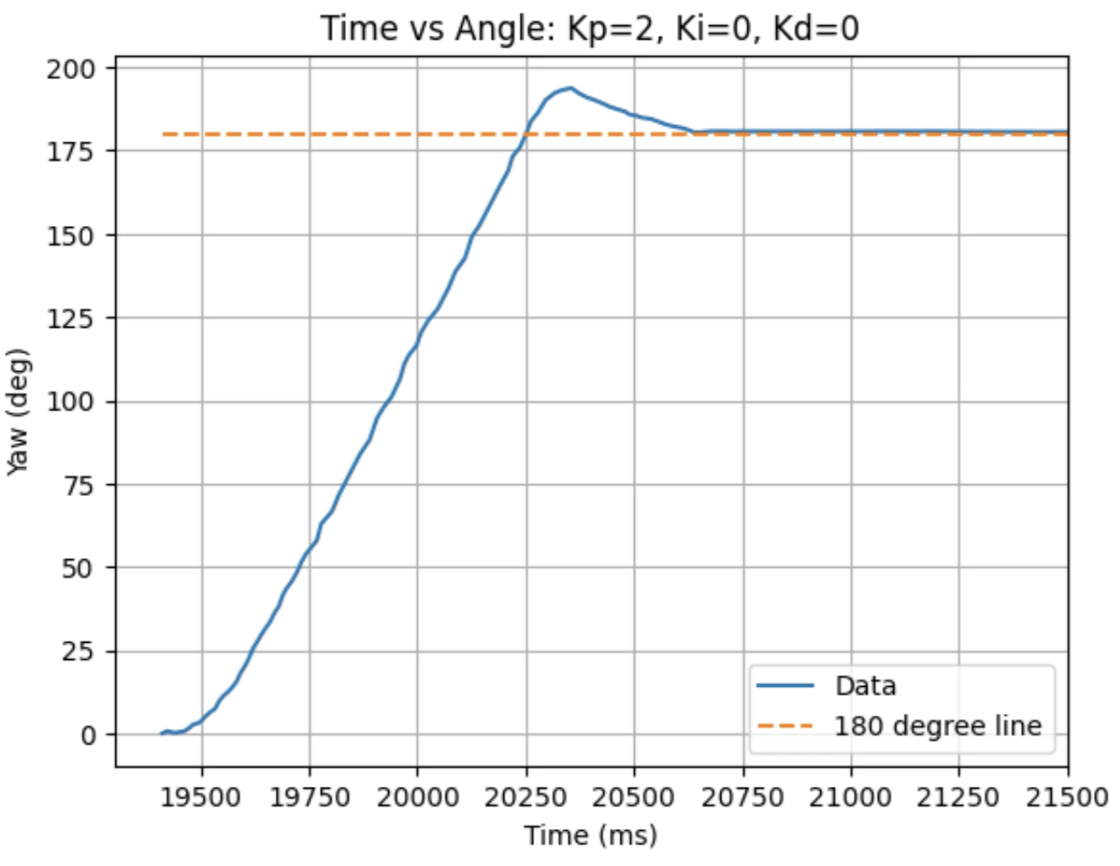
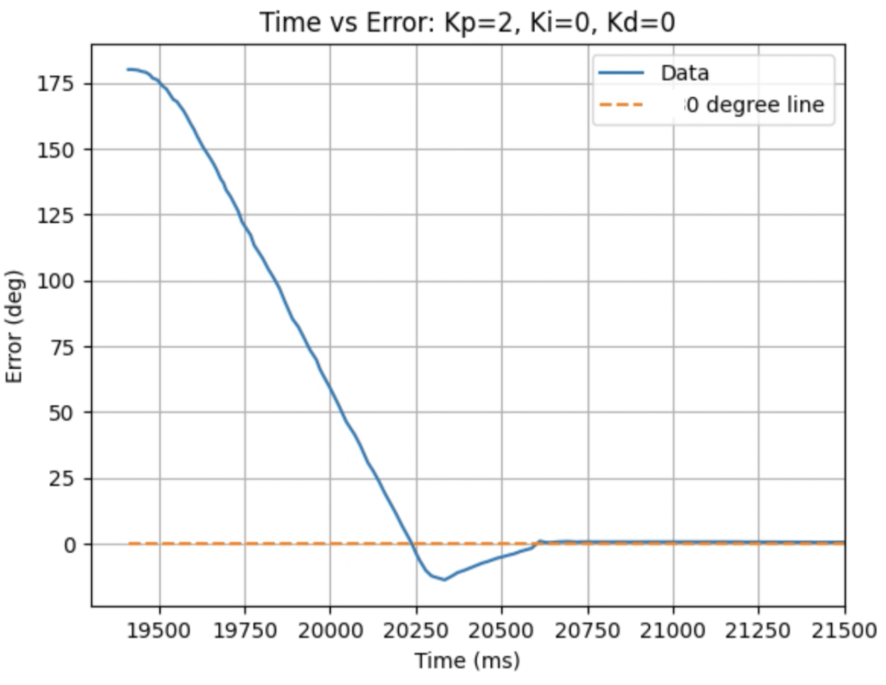
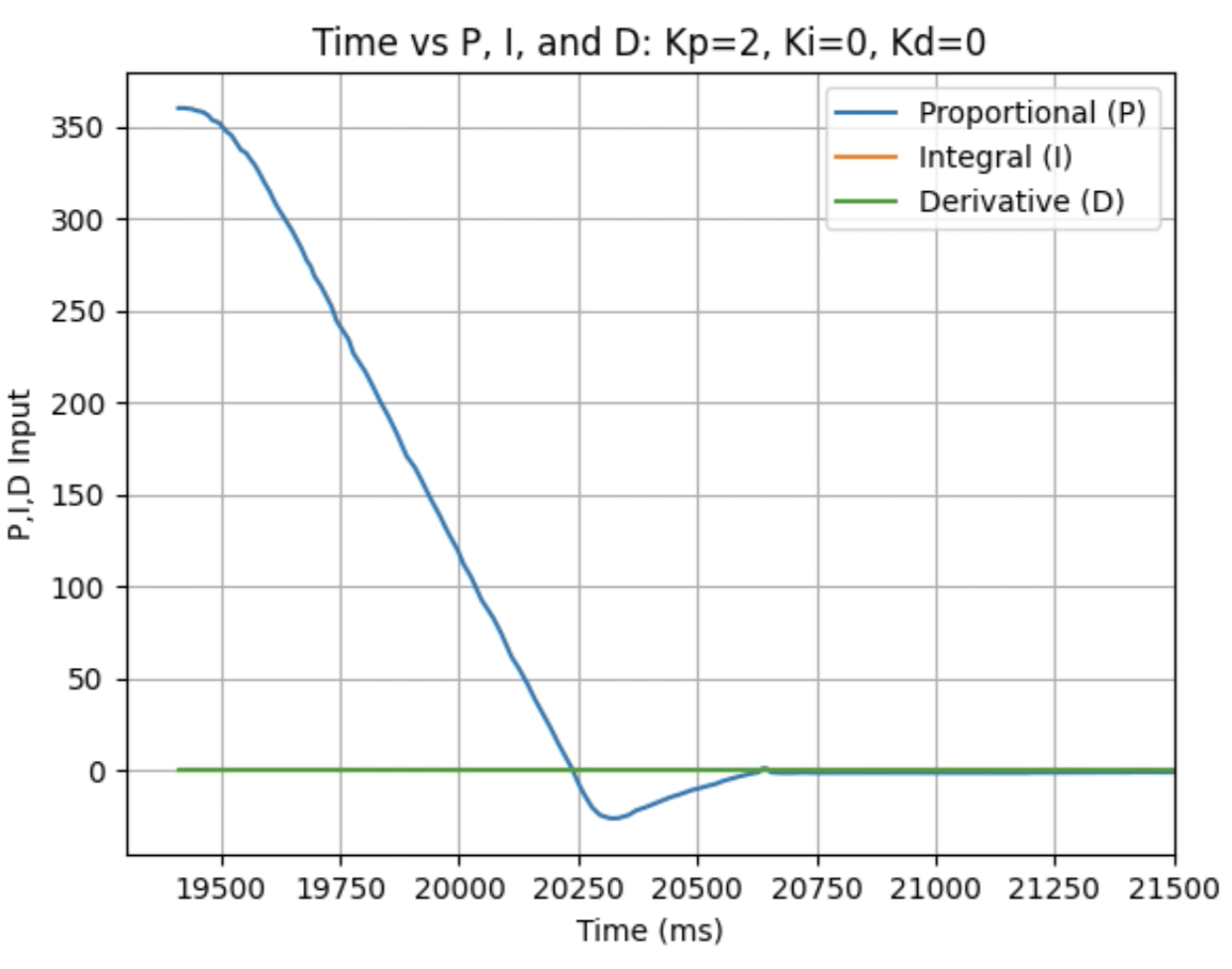
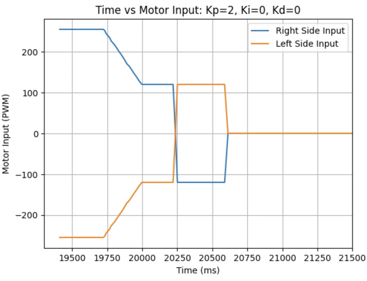
Trends that can be observed include, as the value for Kp increases the amount of time the robot takes to reach the desired angle decreases, but there is also more overshoot observed. As the value of Kp increases the motor input spends less time at the lower limit value of 120. For example, it is noticeably observed that for Kp = 1 the motor quickly reach the input value of 120 and remains at that value until the desired angle is reached. For Kp = 2 the motors start at the upper bound of 255 and then decrease to the lower limit of 120 before reaching 180 degrees. I choose a value of Kp = 2 to then move to testing the proportional and integral controllers together.
5000 Level Task: Integral Control (Ki) and Wind Up Protection
The next step involved using the proportional controller (with Kp = 2) and the integral controller to increase the speed of rotation and to achieve a small amount of oscillation at the desired angle. The integral controller is the constant Ki multiplied by integrated error over time. As time increases the integrated error increases, resulting in a greater contribution of the integral controller. To prevent the integral controller component from increasing continuously, wind up protection was implemented. If the value of Ki mulitplied by the time integrated error is greater than 200 or less then -200, then the KiIntegral is set to be 200 or -200 and does not further increase/decrease. The code for the proportional and integral controller is below.
Below are graphs for the tested values for Kp and Ki.
Graphs for Kp = 2 and Ki = 0.05:
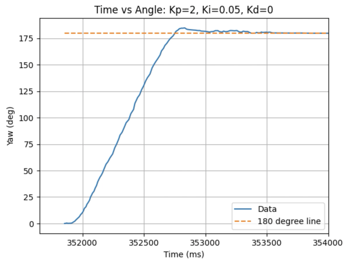
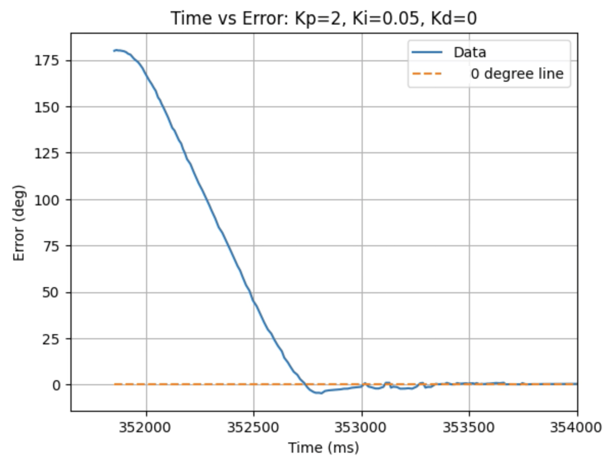
Trends that can be observed include, as the value for Ki increases the amount of oscillation and overshoot of the robot at the desired angle increases. The motor input for all tested values starts at the maximum of 255 before decreasing to a value of 120 before reaching the desired angle. For a value of Ki = 0.01 there is minimal overshoot and oscillation and a value of Ki = 0.05 also results in minimal overshoot but slightly more oscillation. For Ki = 0.1 there is more oscillation before reaching the desired angle and for Ki = 0.2 the oscillation continues for a longer amount of time. I choose a value of Ki = 0.05 to move on to testing the proportional, integral, and derivative controllers together.
Derivative Control (Kd)
Derivative Calculation: Lowpass Filter
The final derivative calculation used the previous gyroscope output combined with a low pass filter with an alpha of 0.3055 to remove some of the noise. The calculation for alpha is found below along with the final code to find the derivative control.
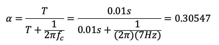
I tested a serives of Kd values to find where the overshoot was reduced. The final derivative calculation resulted in the spike and the noise being removed as can be seen in the below graphs.
Graphs for Kp = 2, Ki = 0.05, and Kd = 0.05:
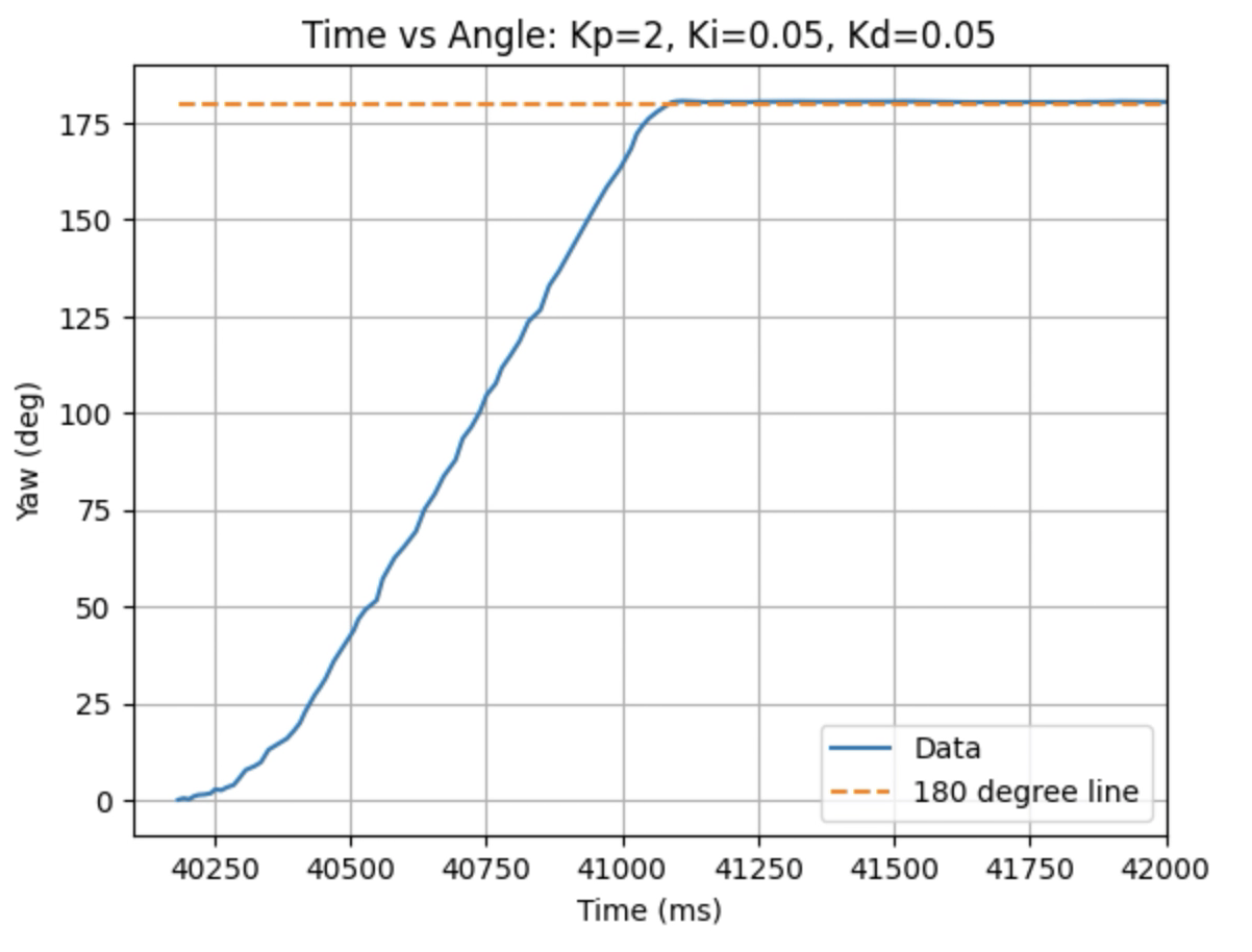
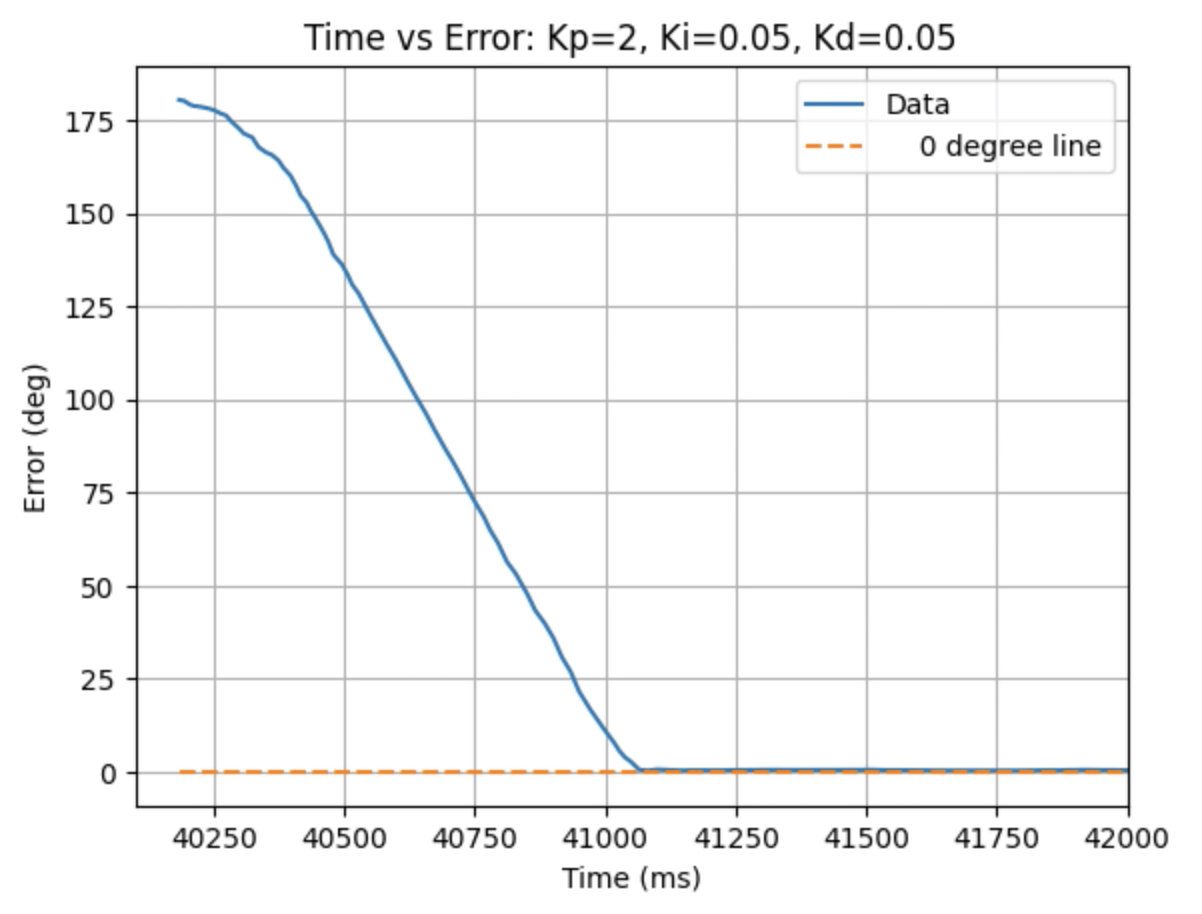
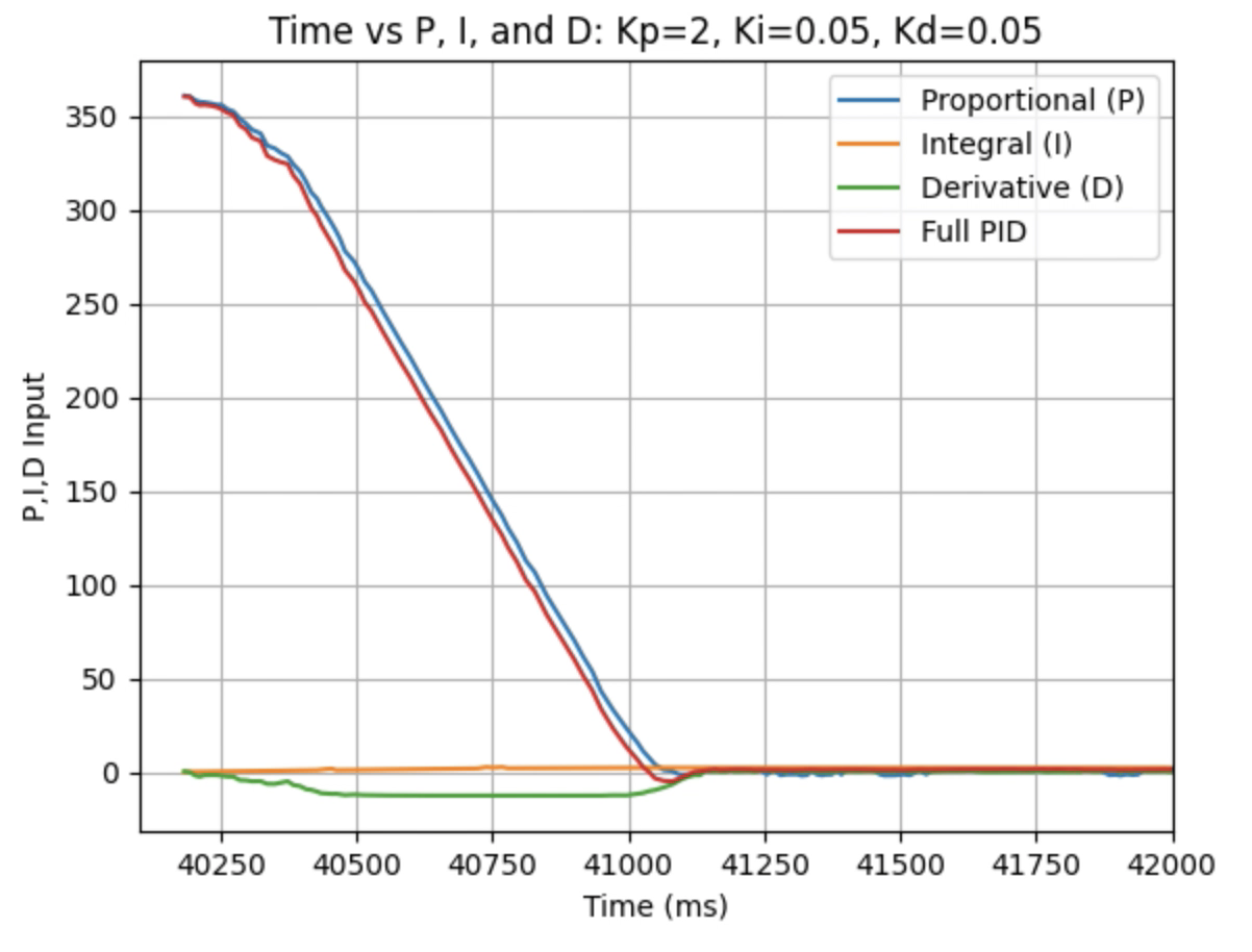
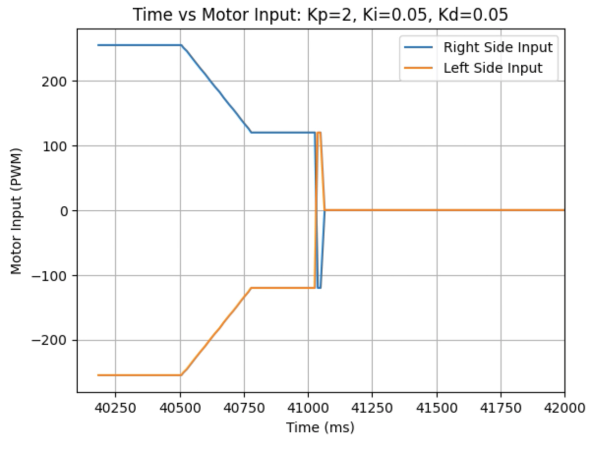
I choose a final value of Kd = 0.05 as the robot did not overshoot the desired angle of 180 degrees.
Below is a video of the robot turning +180 degrees at Kp = 2, Ki = 0.05, and Kd = 0.05:
More Videos
Below is a video of the robot at 0 degrees:
I also tested negative angles. Below is a video of the robot turning -90 degrees:
Lab 5: Linear PID Control and Linear Interpolation
The objective of the lab to to gain experience working with PID controllers. Labs 5-8 detail PID, sensor fusion, and stunts. This lab is focused on using a PID controller for position control of the robot.
PID Control Explaination
For this lab a PID controller will be used for position control of the robot. The below equation from the course Lecture 7 is used to compute the value for the PID controller:
This equation uses the error e(t) (difference between the final desired value and the current value) in proportional, integral, and derivative control to calculate the new PID input value u(t). For this lab the error is the difference between the desired distance from the wall (1ft) and the robots current distance from the wall. The calculated PID input value is related to the robots speed. Proportional control multiplies a constant Kp by the error. Integral control multiplies a constant Ki by by the integral of the error over time. Derivative control multiplies a constant Kd by the rate of change of the error.
Lab Tasks
Final Code For While Loop And Added Functions
Lab 5 Full CodeThe above link has the full final version of the code used during the lab to collect distance measurements, extrapolate distance measurements, and move/stop the robot. I attached the link for my own reference in the future. The below steps show how and why I wrote each piece of the code.
Position Control
For the position control task the robot drives as fast as possible towards a wall and stops when it is 1ft away from the wall. The ToF sensor on the front of the robot will be used to determine the distance the robot is from the wall. The implemented PID control is also shown to be robust to changing conditions including starting distance and floor surface.
Proportional Control (Kp)
The first control input I worked on was the Kp input for proportional control. I estimated the value to be around 0.06899 by using the below equation to solve for the PWM values. I wanted to minimize overshoot, so to find the value for the error I subtracted the final desired distance from the maximum error based on the ToF sensor readings. The equations used can be found below:
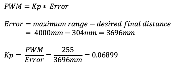
The initial loop used to find the PID value is:

First the time difference (dt) is found and then the error is calculated based on the current distance and desired stopping distance. After the error is calculated the integral and derivative terms are solved for (both are 0 in this step). These PID equations were also used during the next step to find the Kd value for derivative control.
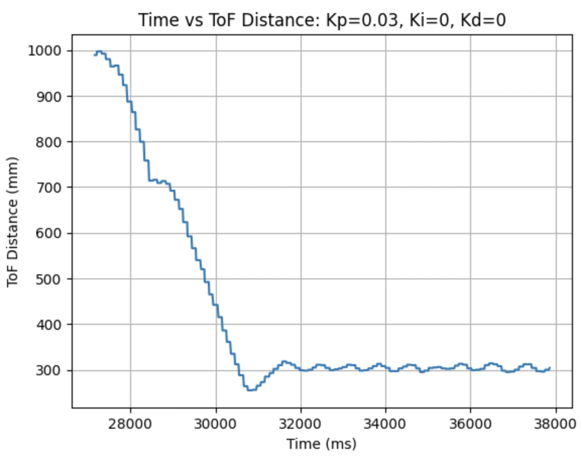
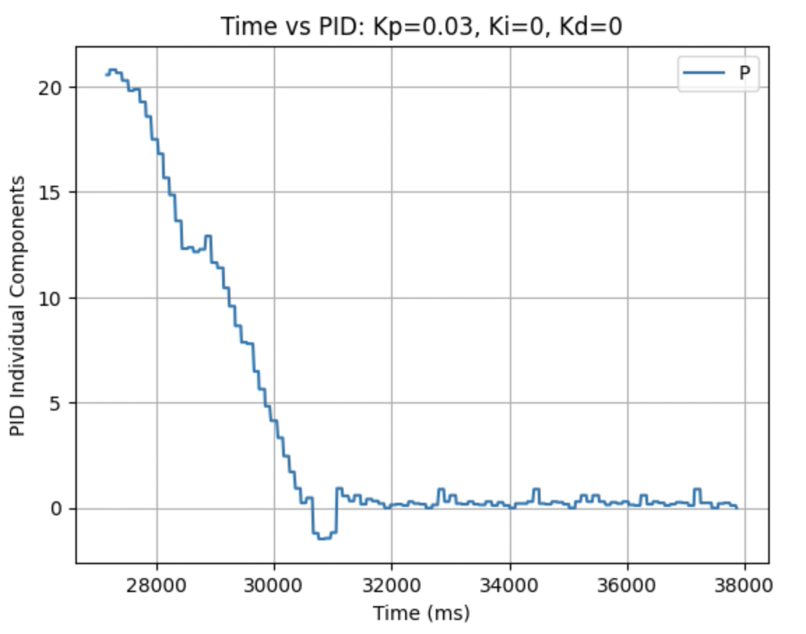
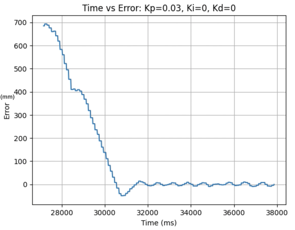
I used the calculated Kp value (0.06899) as an estimate. During the first physical testing of the system I tested a range of Kp values to determine at what point the robot oscillated around 1ft in front of the wall. Two of these Kp values are found graphed below. I determined that the Kp value should be set to 0.03 to minimize the error and oscillation present. The graphs showing Time vs ToF Distance, Time vs P Control, and Time vs Error for Kp = 0.03 can be found below:
Plots for Kp = 0.03:
Video for Kp = 0.03:
Larger Kp values resulted in the robot moving faster and having more error in the final position. Kp = 0.03 was the smallest value for Kp that resulted in the robot completing the full motion. For this first task I wanted to reduce oscillation, rather than achieve a faster speed and moved to the next step using Kp = 0.03. I focused on achieving a faster speed when tuning the integral Ki value, and prevented overshoot when tuning the derivative Kd value.
Derivative Control (Kd)
The next task I worked on was tuning the Kd value using proportional control and derivative control at the same time. I wanted to prevent overshoot and any oscillation of the robot. I increased the Kd value until the overshoot was reduced and the robot stopped at the 1ft desired distance from the wall. This Kd value was found to be Kd = 5. A video showing the robot at Kp = 0.03 and Kd = 5 is below:
Derivative Kick and Low Pass Filter:
For this task the ending setpoint distance does not change, resulting in the error derivative to be continuous. I did not need to implement anything to get rid of derivative kick because there is no changing setpoint. I did consult the reference provided in the lab instructions and read about derivative kick on this website, for future reference.
In addition a low pass filter for the derivative was not implemented as all of the calculated derivative error values were small.
5000 Level Task: Integral Control (Ki) and Wind Up Protection
For the next task I added the integral controller and inputed a Ki value. To start I set Kd to zero and tested a value of Ki = 0.00001 and Kp = 0.03. This resulted in the robot moving very fast into the wall. I then decided to decrease Ki until I found a value where the robot would stop in front of the wall, but for each value tested the robot ran into the wall. I then implemented wind up protection for the integral control to prevent the robot from overshooting and running into the wall.
First a distance measurement is taken at the start of the robots motion to determine the total distance the robot needs to move and an integralStop value is set to be half of the total distance travelled. Each loop an if statement checks to see if the error is greater than the integralStop value. If the error is greater then integralStop a new integral value will be calculated. If the value of the integral term multiplied by the set Ki value is greater than 100 then there will be no further increase in the KiIntegral term used to find the PID control. In additon, if the error is smaller then the integralStop value then the new integral value will be set to zero. The integral term is the Ki value multiplied by the time integrated error. Without wind up protection the integral term will continuously increase causing the robot to not stop when the final distance is reached. Below is a video showing the KiIntegral (I) terms continuously increase until stopping at 100. The error term is not changing significantly, but the KiIntegral (I) term continuously increases.
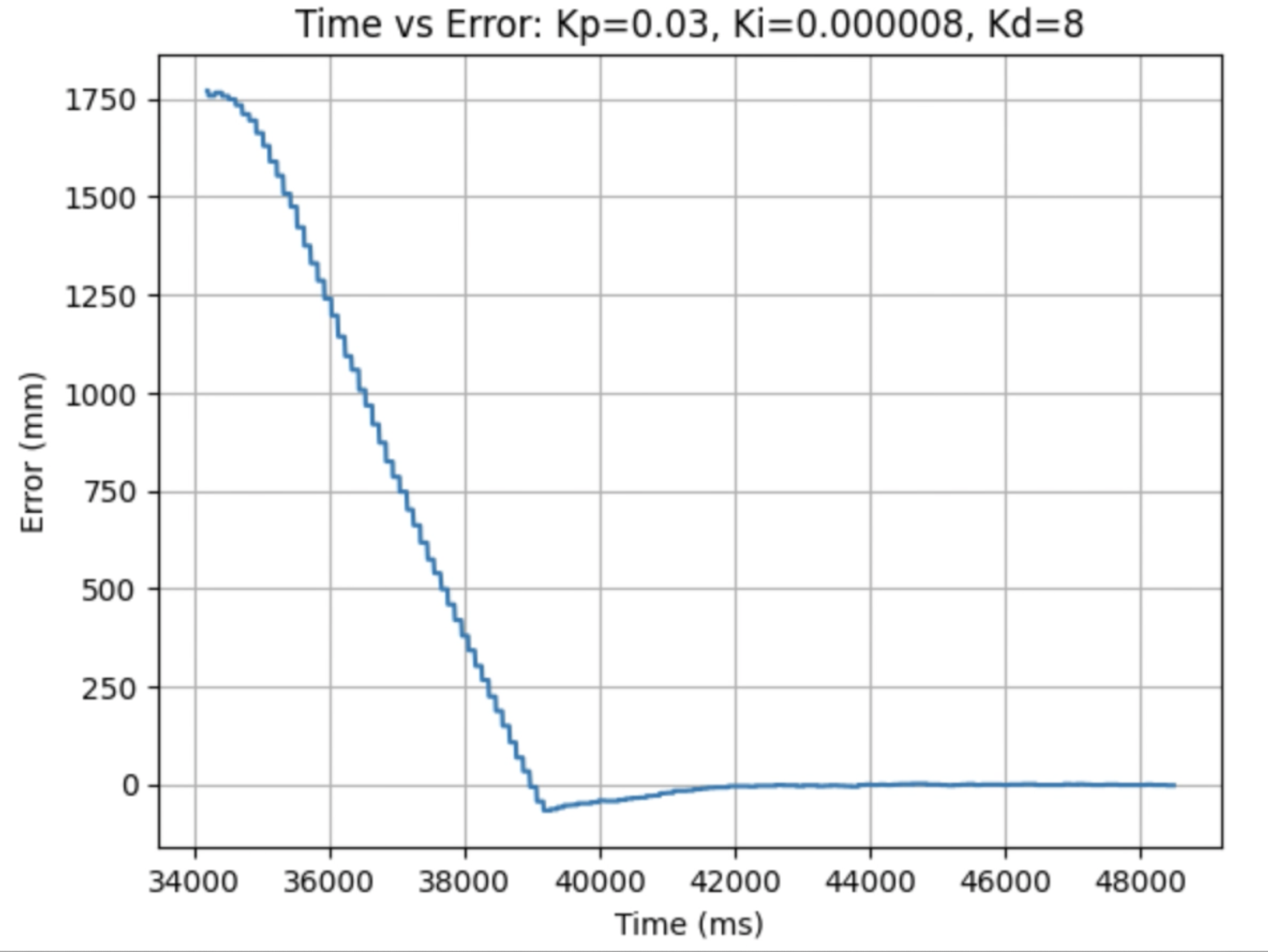
I then added the Kd term found in the previous step. A value of Kd = 5 resulted in more overshoot than I wanted the robot to have. I increased the Kd value until the overshoot was again minimized. This resulted from a value of Kd = 8. For values above Kd = 8 there was no longer a noticable difference in minimizing overshoot. The behavior for Kp = 0.03, Ki = 0.000008, and Kd = 8 can be seen in the three trials below. The robot was started from a distance of 6.5ft.
The three below graphs show the data for Time vs ToF Distance, Time vs Motor Input, and Time vs Error.
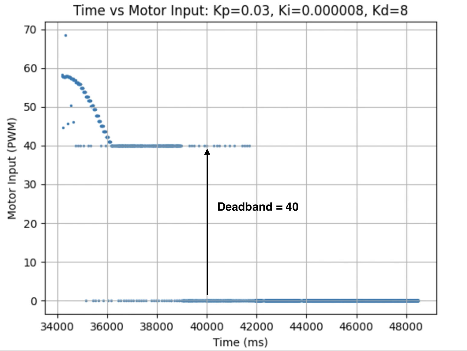
Graph Analysis and Deadband:
The above graphs for the distance and error reading show that there is minimal over shoot and the robot stops at the desired distance of 1ft away from the wall. The graph for Time vs Motor Input shows that the initial motor input is 58 and decreases until a motor input of 40 is reached. The deadband for the motors is 40. Any value between 0.5 and 40 (forward) or -0.5 and -40 (backward) will be set to 40 in order to produce a PWM value that causes the motors to move. I choose a lower bound of 0.5 and -0.5 to prevent the robot from overly moving after reaching the final distance. The functions used to produce forward and backward motion were discussed previously in the section for Proportional Control. When the robot stops the motor input changes to zero.
Maximum Linear Speed:
The maximum linear speed of the robot can be found using the Time vs ToF Distance graph. Using two points on the graph it can be found that (1506mm - 707mm)/(36105ms - 38258ms) = 0.37m/s
Extrapolation
Frequency of Returned ToF Data
As stated previously in the lab in the Range and Sampling Time Discussion section, the sampling period was found to be 100ms, resulting in a sampling frequency of (1/0.1s) = 10Hz for distance measurements.
Speed of PID Control Loop and ToF Sensor Rate
As stated previously in the lab in the Range and Sampling Time Discussion section, The PID loop runs at around 8ms, which is faster than the ToF sensor produces new distance readings. Extrapolation will be used to estimate the distance when new data is not available using past ToF distance readings.
Calculate PID Control Every Loop and Extapolate Robot Distance From Past Data Readings
Due to the ToF sensor running slower than the PID loop, extrapolation is used to estimate the distance using past data points. Below is the extrapolation equation:
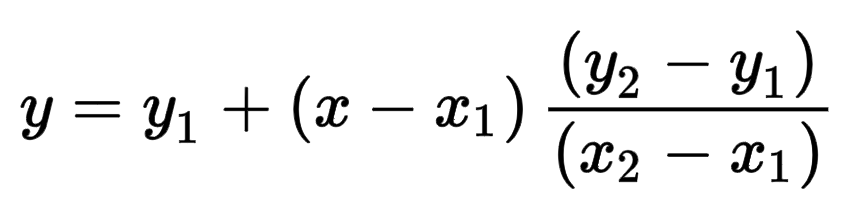
This equation was implemented in the Arduino code. An if statement checks if the ToF distance sensor has a new distance reading. If the sensor has a new distance reading then that point is added to the distance_data array and the current time and distance are stored in time1 and dis1 variables. The previous time and distance from the last time there was a new distance measurement are stored in the time2 and dis2 variables. If there is no new distance reading the extrapolation equation is used.
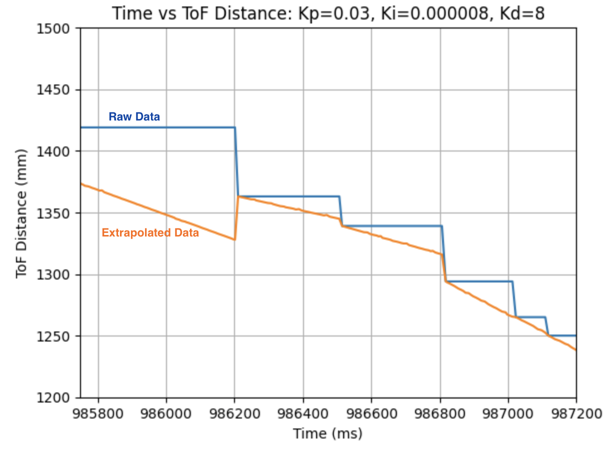
Below is a graph for the raw and extrapolated distances. The graph is zoomed in to show that the extrapolated data (orange) readjusts to the raw data reading (blue) every time there is a new distance measurement. In the next section I ran tests using the extrapolated data.
Lab 4: Motors and Open Loop Control
The objective of the lab is to control the car using open loop control, rather than the manual controller. Two dual motor drivers will be connected to the car's motors and the Artemis board. The dual motor drivers will be used to control the movement of the car.
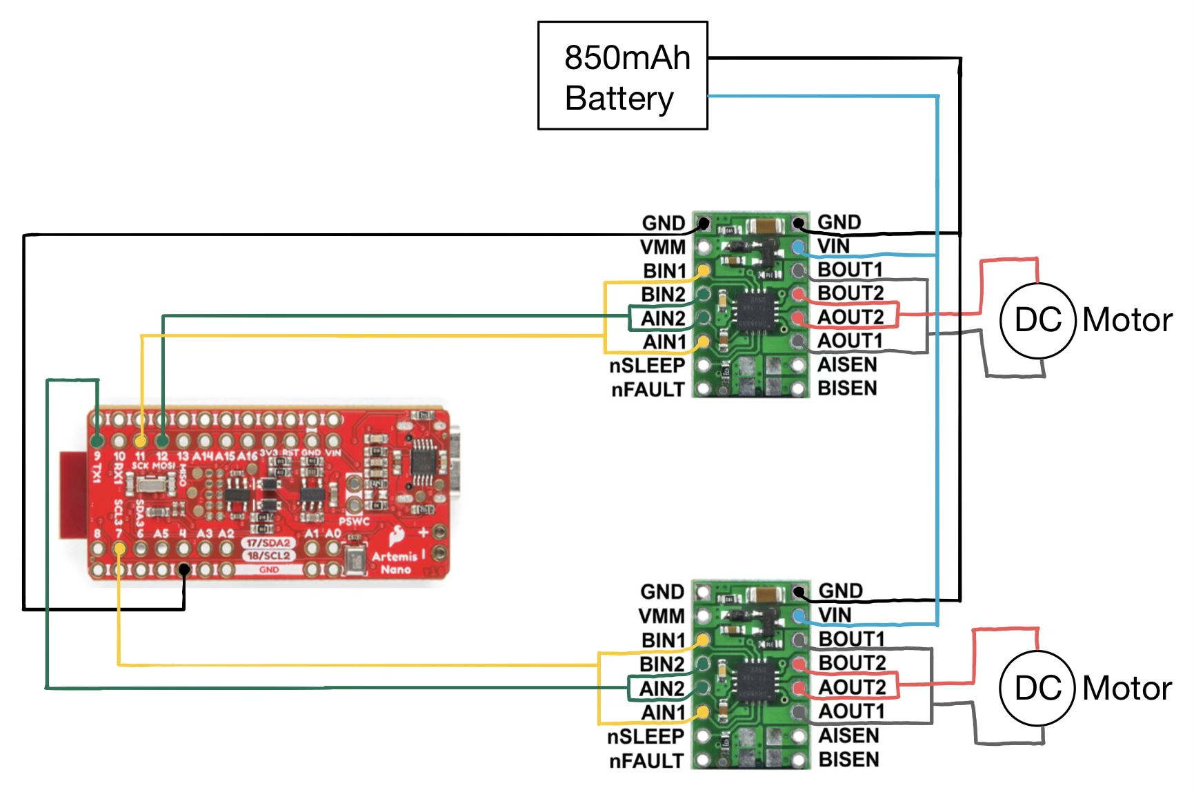
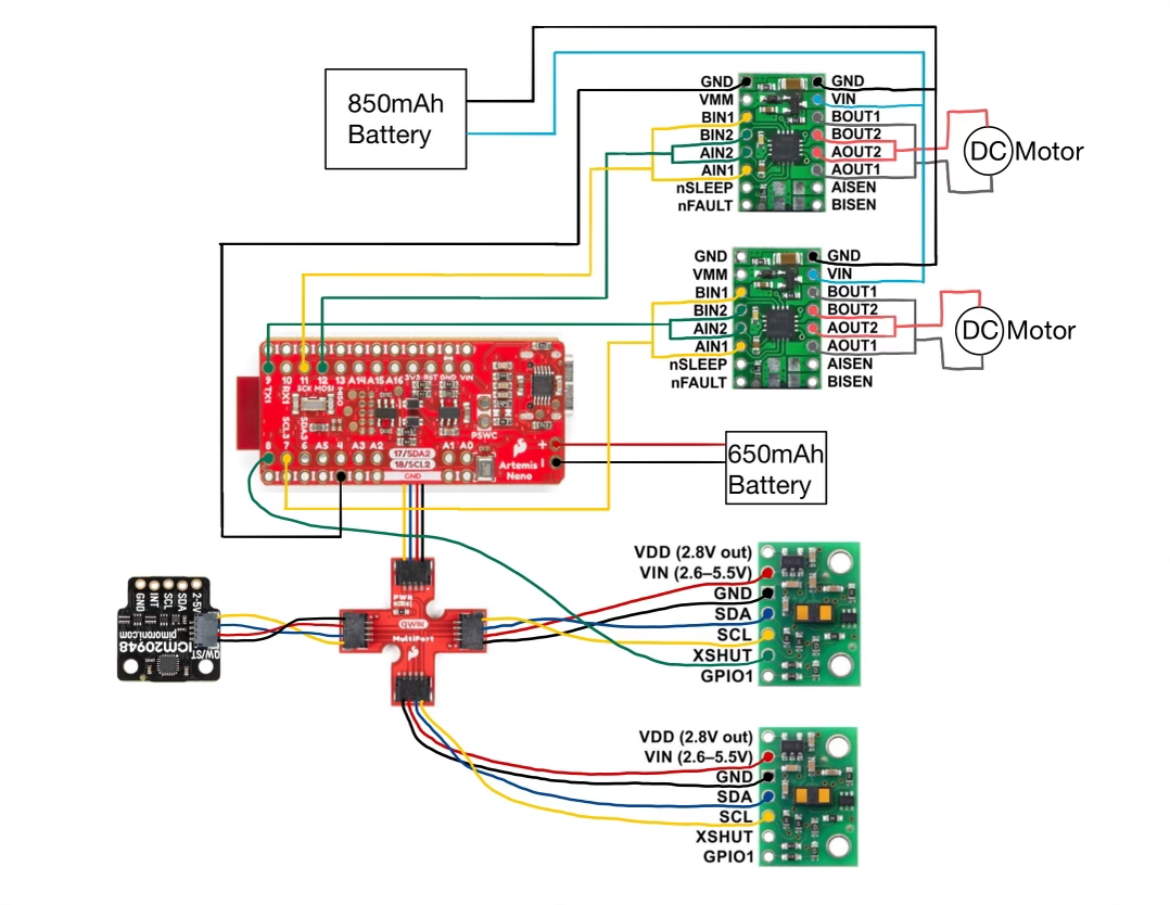
Sketch Of Wiring Diagram
Below is a wiring diagram for the two dual motor drivers connected to the Artemis board, DC Motors, and 850mAh battery. The two VIN pins and the two GND pins on both dual motor drivers are connected together and then connected to the 850mAh battery. The GND pin of one of the dual motor drivers is connected to the GND of the Artemis board. There is a bridge between the BOUT1 and AOUT1 pins of the dual motor driver that is then connected to the DC motor. There is also a bridge between the BOUT2 and AOUT2 pins of the dual motor driver that is then connected to the DC motor. There is a bridge between the BIN1 and AIN1 pins on the dual motor driver and there is also a bridge between the BIN2 and AIN2 pins. On the dual motor driver that connects the drivers to the ground of the Artemis board (top dual motar driver in sketch below), the bridge between BIN1 and AIN1 is connected to pin 11, and the bridge between BIN2 and AIN2 is connected to pin 12. On the other dual motor driver (bottom dual motor driver in sketch below) the bridge between BIN1 and AIN1 is connected to pin 7, and the bridge between BIN2 and AIN2 is connected to pin 9. The pins used in this lab were chosen from the remaining pins on the Artemis board (after the previous lab). The parallel-couple of the two inputs and two outputs on each dual motor driver allows for twice the average current to be delivered without overheating.
Lab Tasks
Testing The Circuit With The Oscilloscope and Power Supply
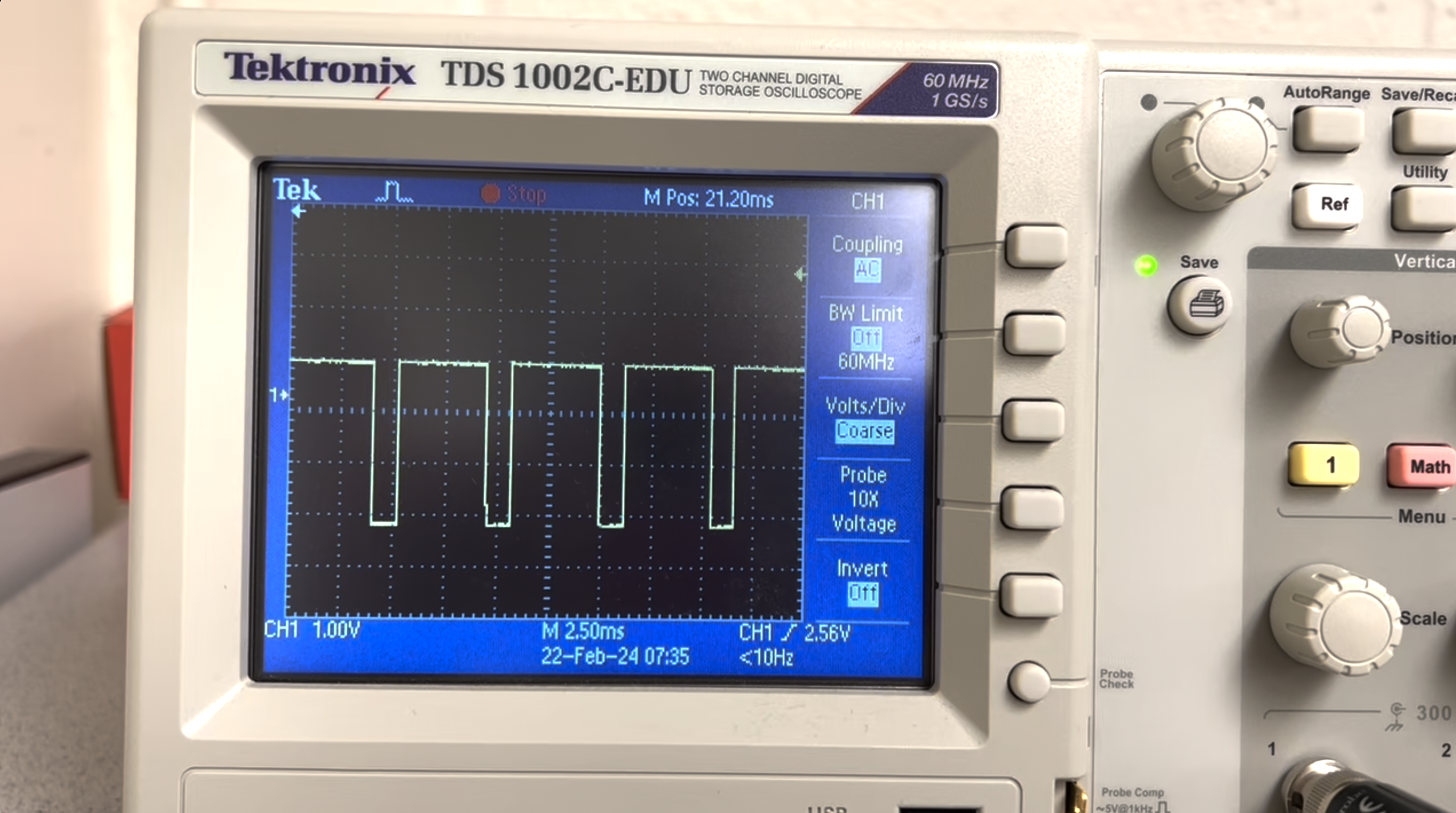
Power Supply Setting And Oscilloscope Discussion
The voltage of the 850mAh battery is 3.7V. In place of using the battery, a power supply was used. The output of the power supply was set to 3.7V to represent the battery power that will be used later on during the lab. Each pin was tested independently of each other. In the Arduino IDE code, one pin was set to have an output of 200, while the other pins all had an output of 0. This was repeated for all four pins. The positive output voltage to the motor was displayed on the oscilloscope and indicated a constant voltage output at each time. The PWM values show that power can be regulated on the motor driver output.
Channel 3 of the power supply was used. 3.7V was used to test the motor driver circuit.
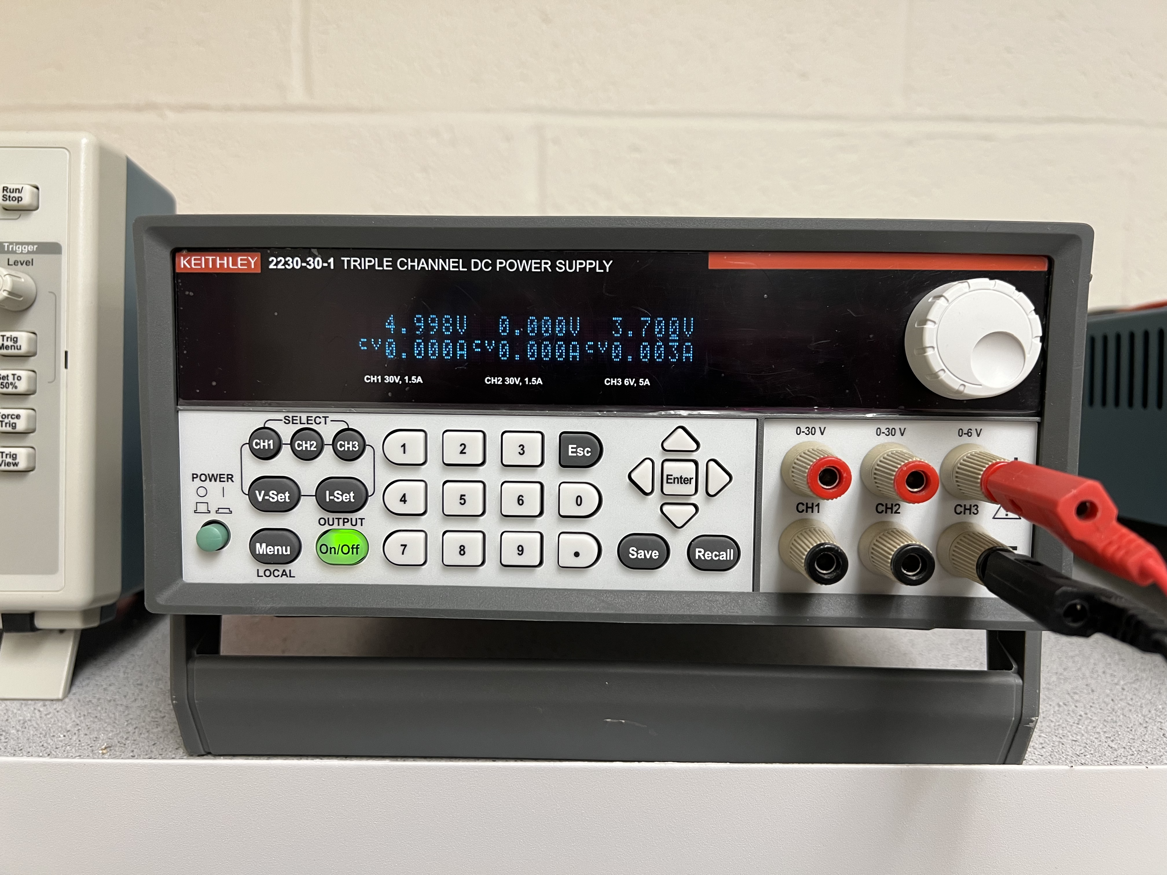
Picture of the oscilloscope output:
Testing The Robot Wheels
Video Of Wheels Spinning (Each Side Of Robot)
The wheels on each side of the robot were tested individually at two different output values. The power supply used at the beginning of the lab (3.7V) was used to power the motors. Pins 7, 9, 11, and 12 were tested at output values of 50 and 200. While testing each side of the robot I observed the direction and speed that each wheel turned. The wheels rotated faster for the higher output at 200 compared to the output at 50. For the higher output value of 200, the wheels reached the final set speed faster compared to the lower set speed. When rotating at 50 the wheels took longer to start rotating. From the perspective of the videos pin 7 rotates counter clockwise and pin 9 rotates clockwise. Pin 7 and pin 9 move the wheels on the same side of the robot in different directions. In addition, from the perspective of the videos pin 11 moves clockwise and pin 12 moves counter clockwise. Pin 11 and pin 12 move the wheels on the same side of the robot in different directions. To consolidate the report, all of the videos taken can be found in this folder: Folder Link Below are videos of pin 12 and pin 9 with an output value of 200.
Pin 12 with an output of 200:
Pin 9 with an output of 200:
The Arduino code to test the wheels is found below. One pin was set to have an output value of either 50 or 200 and all other pins were set to have an output value of 0. This is the same code that was used in the previous section to test if the circuit was working properly before sautering to the motors.
Video Of All Wheels Spinning
After testing each side of the robot, all of the wheels were tested at the same time. The 850mAh battery was used to power the motors instead of the power supply. The below video shows both sides rotating while the motors and Artemis board are both connected to their respective batteries.
The Arduino code to test the wheels on both sides of the robot is found below. Pins 9 and 12 were set to have an output of 200 and pins 7 and 11 were set to have an output value of 0. This is the same code that was used in the previous section to test both sides of the robot individually.
Picture Of All Components On Car
Below is a labeled picture showing all components on the robot. Including the 650mAh battery, Artemis board, IMU, two ToF sensors, two motor drivers, and a breakout board. The 850mAh battery to power the motors is on the other side of the robot.
Below is a diagram of the entire wiring that is used on the robot:
Lower Limit PWM And Open Loop Control
Lower Limit PWM Value Discussion
The lower limit PWM value is the lowest output value that a pin can be set to that will still result in continuous motion of the robot. The wheels on one side of the robot were tested, while the wheels on the other side remained stationary. The lower limit PWM for pin 11 (right side) was found to be 59. The lower limit PWM for pin 7 (left side) was found to be 50.
Pin 11 (Right Wheels) with an output of 59:
Pin 7 (Left Wheels) with an output of 50:
I also found the PWM value for both wheels when they are being used together, starting when the robot is stationary. The output value was found to be 35 for both wheel sides. The video showing the robot moving when both wheels (pins 11 and 7) have an output value of 35.
Calibration Demonstration
The wheels of the robot do not spin at the same rate and a calibration factor needed to be implemented. The below video shows the robot moving in a straight line, starting at 7 feet and then continuing past the end of the tape measure. For the demonstration, pin 11 was set to an output of 60 and pin 7 was set to an output of 70. In addition to the below video, the robot was run multiple times at varying input values. My first tested value was pin 11 at an output of 60, which is close to the found PWM value from the previous step. When pin 7 was set to an output of 51, the robot continuously moved towards the left. Through trial and error I found that an output of 70 for pin 7 kept the robot moving in a straight line. I used these found values for reference during future tests: 70/60=1.166666666666667.
I increased the output of pin 11 by 20 for each test and multiplied the value for pin 7 by 1.166666666666667. This incrementation worked for all tested pin 11 and pin 7 values until I reached an output value of 220 for pin 11. The calculated output value for pin 7 should be 257, rounded down to 255 due to 255 being the maximum output value. For this test the robot continuously moved towards the right and the value for pin 7 needed to be lowered to 250 to keep the robot moving straight. Due to this discovery, I decided to also test an output value of 210 for pin 11, the calculated output value for pin 7 should be 245. In order to keep the robot moving straight, and not to the right I needed to reduce the output of pin 7 to 240. The trend shows that after an output of 200 for pin 11 the calibration factor to find the corresponding output value for pin 7 starts to differ.
In addition, as a final test I wanted to determine how low I could set the output values while still having the robot move in a straight line for at least 6 feet. I set the output value of pin 11 to 40 and calculated the output value of pin 7 to be 47. For these output values, the robot moved in a straight line for more than 6 feet. When I set the output value for pin 11 to be lower than 40 the wheels began to stall and hesitate before rotating compared to the other side of the robot. I also included a video at the end of the section showing the wheels spinning.
To produce the robots motion the same Arduino IDE case and Jupyter Notebook command were used from the previous section. The length of the delay was changed depending on how fast the robot moved (to prevent the robot from running into a wall). All of the recorded videos are in this folder.
Below is a graph showing all of the tested values as data points. In addition, I plotted the trendline for all data points, as well as the trendline for all of the data points except for the last two that began to differ from the previous measurements. The slope and y-intercept were also found for each trendline. The calculated slope is the calibration factor. The slope excluding the last two data points, 1.165 is close to the 1.166666666666667 value.

Video showing wheels hesitating when pin 11 (right) has an output of 35 and pin 7 (left) has an output of 41:
I also tested the calibration factor when the robot is going in "reverse" (with the robot moving in the direction away from the ToF sensor on one end). I initially tested the previously found output values with the corresponding pins on each wheel side, with pin 12 having an output of 60 and pin 9 having an output of 70. I found that by doing this the robot moved towards the left. I decided to switch the output values; pin 12 has an output of 70 and pin 9 has an output of 60). The robot moves straight using these output values. I find this interesting as it confirm my previous thoughts about one side of the wheels being slightly misaligned.
Open Loop Code And Video
Below is a video showing open loop control of the robot. In the video the robot moves forward, turn towards the right, moves backward, stops, spins counterclockwise, stops, spins clockwise, and then stops. I used output values found from the calibration graph.
Lowest PWM Value Speed Discussion
The lowest PWM value for each side of the robot was found by running the robot with an initial output of 60 for pin 11 and 70 for pin 7 to correspond with the found calibration values. The robot ran with these outputs for 3 seconds and then all pin outputs were set to zero expect either pin 11 or pin 7. Either pin 11 or pin 7 remained turned on for another 3 seconds, but decreased to a lower output value. I ran the robot multiple times to determine at what output value the robot no longer moved. It was determined that for pin 11 the lowest PWM output is 35 and for pin 7 the lowest PWM output is 33. The videos for each pin can be found below.
Pin 11 with a lowest PWM value of 35:
Pin 7 with a lowest PWM value of 33:
In addition, the lowest combined wheel PWM value was found when both wheels were being used at the same time. The output value for both wheels (pin 11 and pin 7) is 25 when the robot is already moving. The robot was initially run with an initial output of 60 for pin 11 and 70 for pin 7 for 1.5 seconds and then both wheels decreased to an output of 25 for 5 seconds. Below are two videos. One video shows the final output at 25 (the robot moves until the total set time of 5 seconds is over). The other video shows the robot stop before the 5 seconds is over and the motors stall when set to an output of 24, confirming the lower limit PWM value of 25 to keep the robot moving.
Both Wheels: Lower Limit PWM of 25:
Both Wheels: Tested value of 24:
Lab 3: TOF
The objective of the lab is to connect the time of flight (TOF) sensors to the Artemis board.
Note The I2C Sensor Address
From the datasheet it was found that the I2C sensor address for the ToF sensor is 0x52. The two ToF sensors have the same address and one of the addresses will need to be changed in order to receive data from both sensors at the same time.
Approach To Using Two ToF Sensors
To use two ToF sensors, the XSHUT pin will be used to connect one of the ToF sensors to pin 8 on the Artemis board. The XSHUT pin will be set to LOW and then the I2C sensor address will be changed for the other ToF sensor that is on. After the I2C address has been changed the XSHUT pin will be set to HIGH, turning the other TOF sensor back on. This will allow for both ToF sensors to be used in parallel.
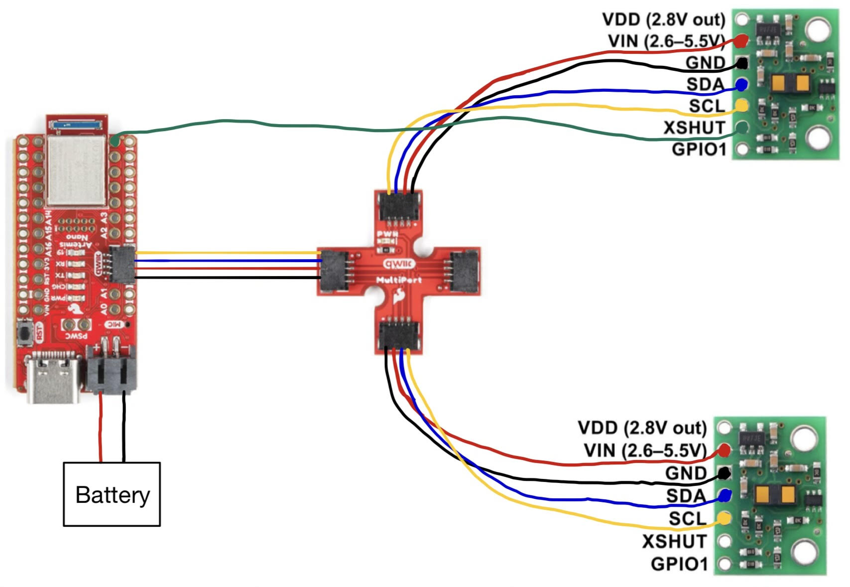
Sketch Of Wiring Diagram
Lab Tasks
ToF Sensor Connected To QWIIC Breakout Board
The Artemis board was powered using a battery:
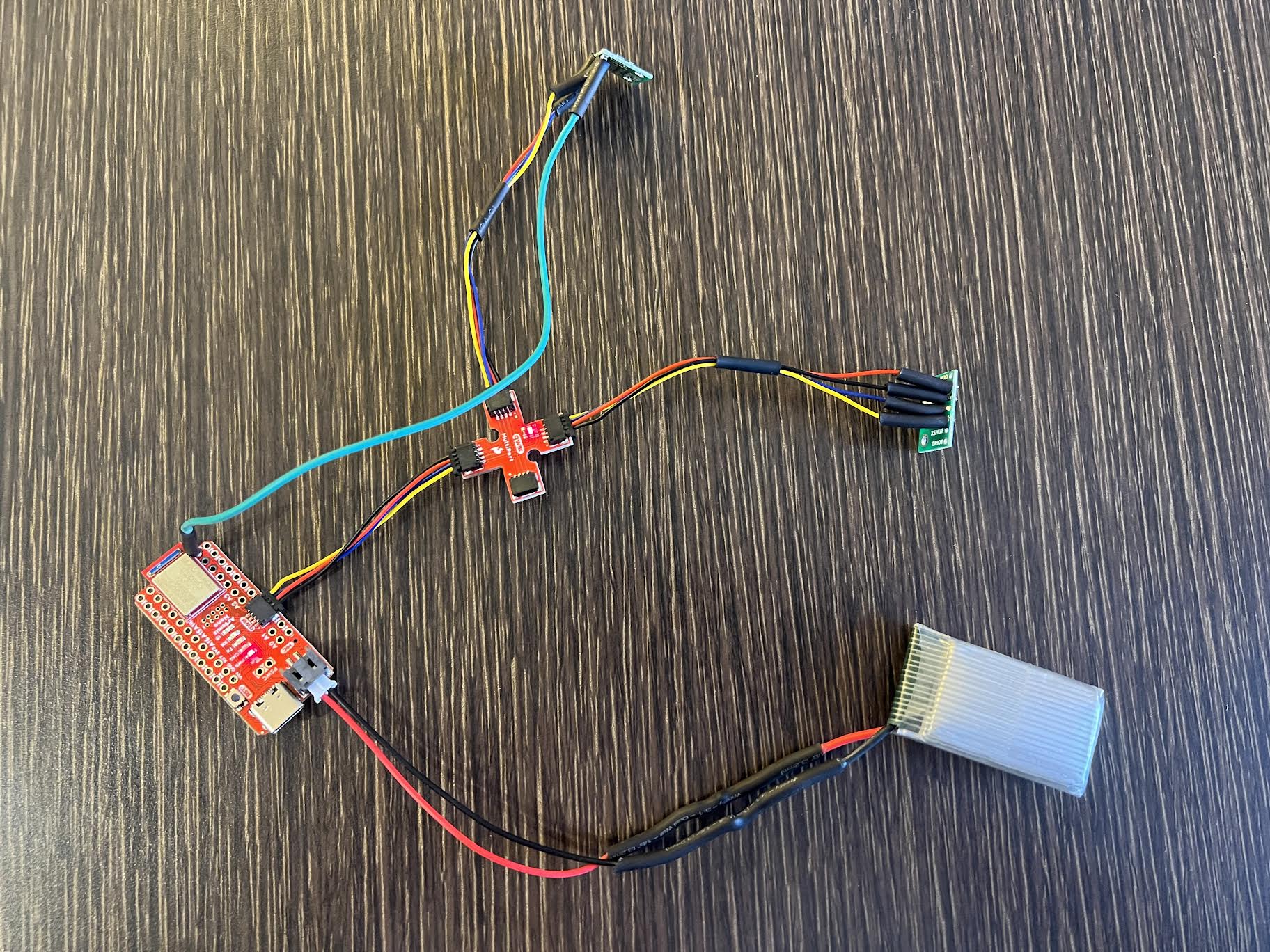
ToF sensors connected to the QWIIC breakout board:
Artemis Scanning For I2C Device
The SparkFun VL53L1X 4m Laser Distance Sensor Library was installed on Arduino IDE. The code to find the I2C address: File->Examples->Apollo3->Wire->Example05_Wire_I2C.ino
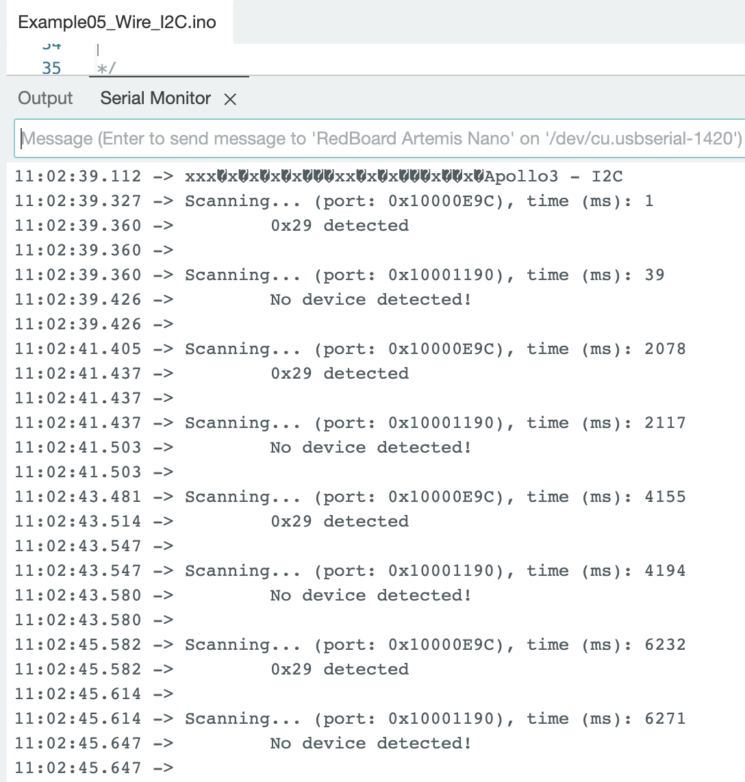
One ToF sensor was connected during the scan. The sensor had an I2C address of 0x29. In the datasheet for the ToF sensor, the listed I2C address is 0x52. The Example05_Wire_I2C.ino code returned an address of 0x29. This is a result of the binary for address 0x52 (binary: 0b01010010) being shifted to the right, resulting in an address of 0x29 (binary: 0b00101001). The rightmost bit is ignored because the bit identifies if data is read/write.
Sensor Data With Chosen Mode
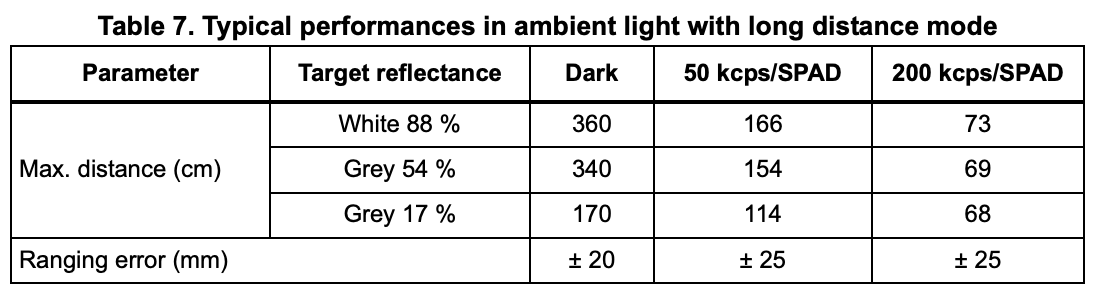
Sensor Mode Discussion
The ToF sensor has two modes: (.setDistanceModeMedium(); //3m has been removed)
Information from the datasheet shows that the short mode can only reach up to 1.3m and is the most resistant to ambient light. The long mode can reach up to 4m but is very sensitive to ambient light, which decreases the distance to 0.73m. The timing budget range for the short mode is 20ms - 1000ms. The timing range for the long mode is 33ms - 1000ms. Short mode has greater accuracy and less sensor noise compared to the long mode. While it would be beneficial for a robot that needs to sense objects farther away to use the long mode, for this lab I am prioritizing accuracy and choose to test the short mode.
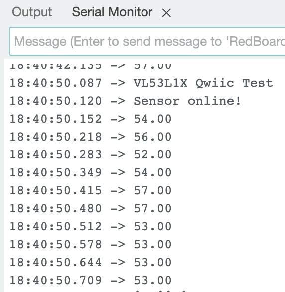
Testing .setDistanceModeShort();
The ToF sensor was first tested using the File->Examples->SparkFun_VL53L1X_4m_Laser_Distance_Sensor->Example1_ReadDistance.ino This code was modified to include the line distanceSensor.setDistanceModeShort(); in the setup to choose the short mode for the ToF sensor.
ToF Sensor Setup:
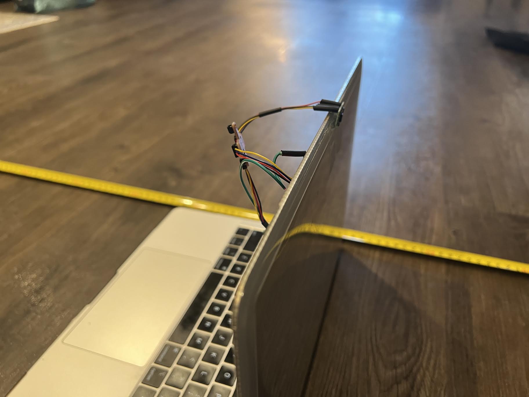
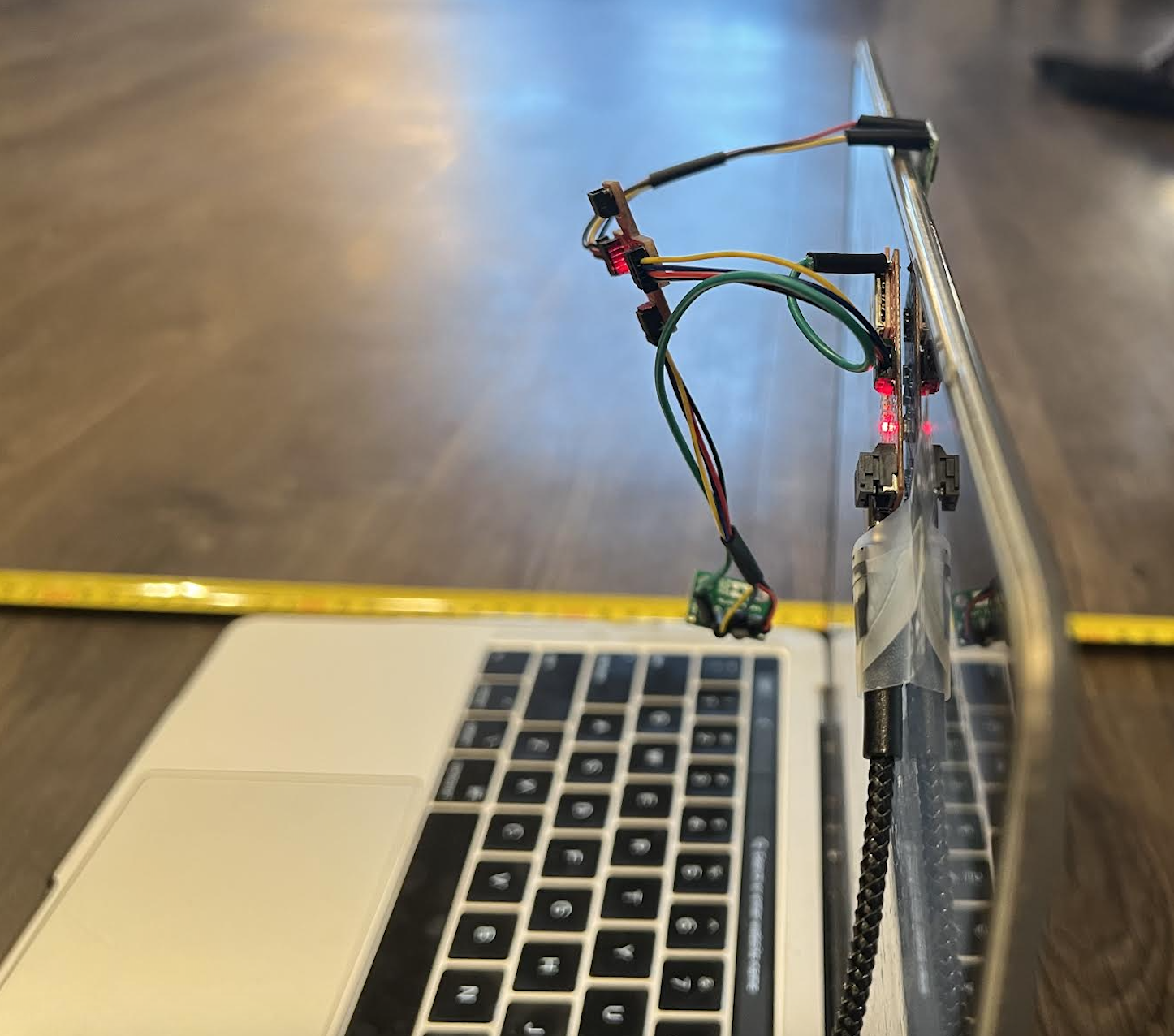
Sensor Range:
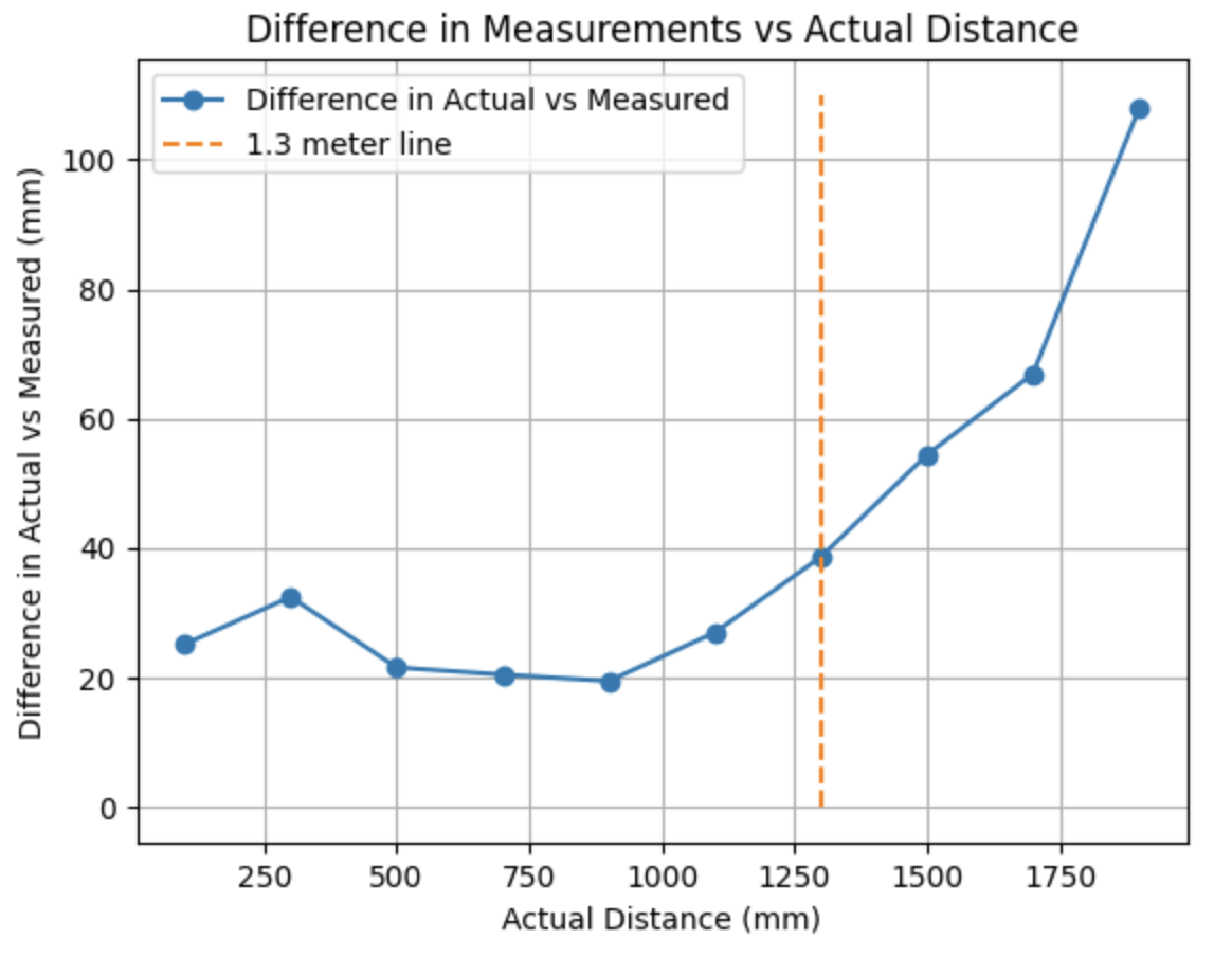
In the datasheet it is stated that the short mode for the ToF sensor has a range up to 1.3m. To test the range of the sensor I took an initial measurement at 100mm and continued to take measurements up to 1900mm. The graph below shows the actual distance of the ToF sensor from the wall vs the ToF sensor distance. The plotted measured distance value is the mean value of the ten collected data points. From the graph below it can be seen that after 1.3m the measured values start to differ more from the actual values compared to measured values less than 1.3m.

Accuracy:
The difference in the measured and actual distances was plotted against the actual distances the ToF sensor was from the wall. When the ToF sensor is less than 1.3m from the wall, the difference is between 18mm and 40mm. After 1.3m the difference in the measured vs actual distance increases.
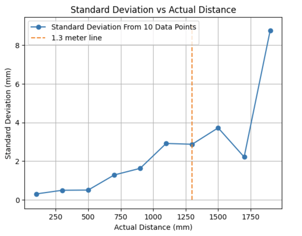
Repeatability:
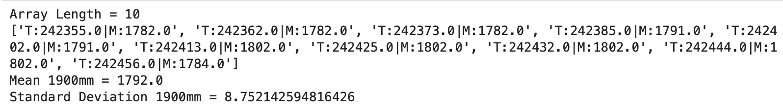
The standard deviation vs actual distance graph is shown below. The standard deviation is below 3mm for measurements under 1.3m. After 1.3m the standard deviation starts to vary and the standard deviation at 1900mm is 8.75mm.
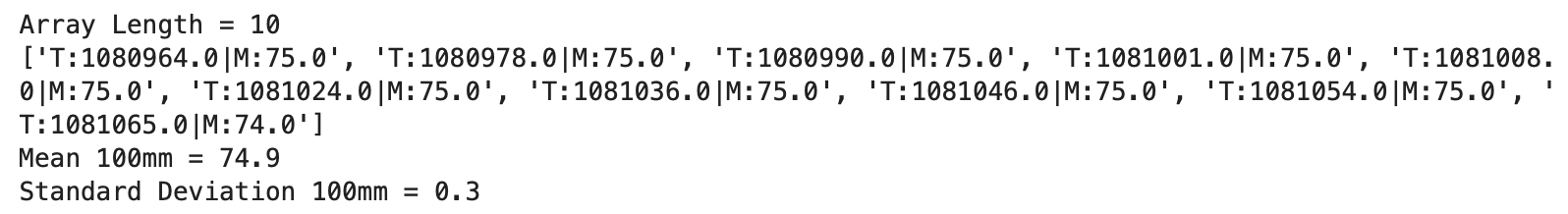
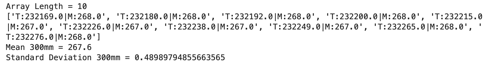
Below are the time and measured distance arrays:
100mm: 9 measurements at 75mm, 1 measurement at 74mm
300mm: 6 measurements at 268mm, 4 measurements at 267mm
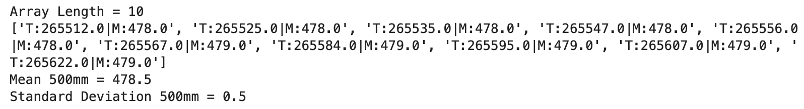
500mm: 5 measurements at 478mm, 5 measurements at 479mm
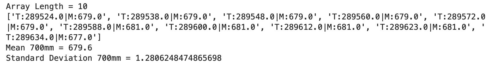
700mm: 5 measurements at 679mm, 4 measurements at 681mm, 1 measurement at 677mm
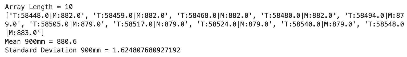
900mm: 4 measurements at 882mm, 5 measurements at 879mm, 1 measurement at 883mm
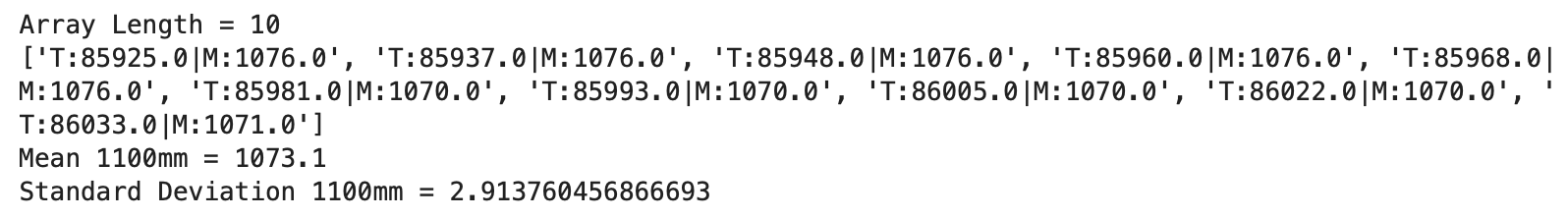
1100mm: 5 measurements at 1076mm, 4 measurements at 1070mm, 1 measurement at 1071mm
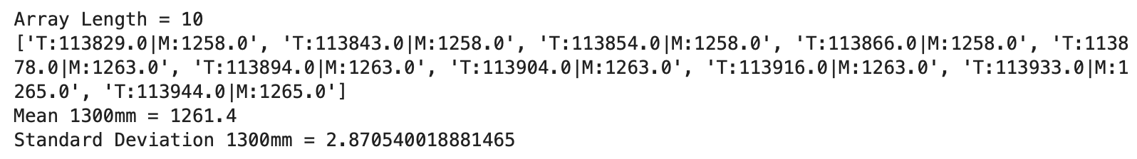
1300mm: 4 measurements at 1258mm, 4 measurements at 1263mm, 2 measurements at 1265mm
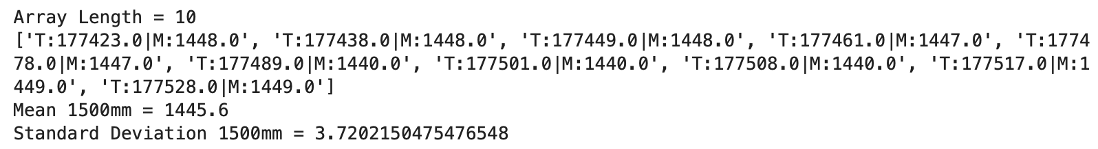
1500mm: 3 measurements at 1448mm, 2 measurements at 1447mm, 3 measurements at 1440mm, 2 measurements at 1449mm
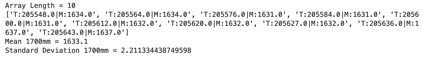
1700mm: 2 measurements at 1634mm, 3 measurements at 1631mm, 3 measurements at 1632mm, 2 measurements at 1637mm
1900mm: 3 measurements at 1782mm, 2 measurements at 1791mm, 4 measurements at 1802mm, 1 measurement at 1784mm
Ranging Time:
The ranging time is the time between each sensor measurement. I commented out all print statements, except the calculated value between the start and end times to allow for code to run as fast as possible. The ranging time was found to be around 55ms.
Two ToF Sensors: Working In Parallel
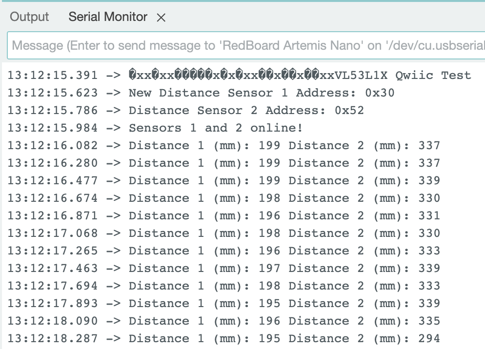
Two ToF Sensors were connected to the Artemis board and Arduino code needed to be written for the two ToF sensors to work in parallel.
The Serial Monitor prints the I2C addresses for both distance sensors to confirm that one of the addresses was changed to 0x30 and the other remains 0x52.
ToF Sensor Speed: Speed And Limiting Factor
Time is continuously printed and distance measurements are only printed when a measurement is available. When the sensors are not collecting data the loop takes around 2ms. When data is being collected the loop takes around 11ms. The longer loop time when collecting ToF sensor data is the limiting factor. The limiting factor is the time needed to record distance measurements.

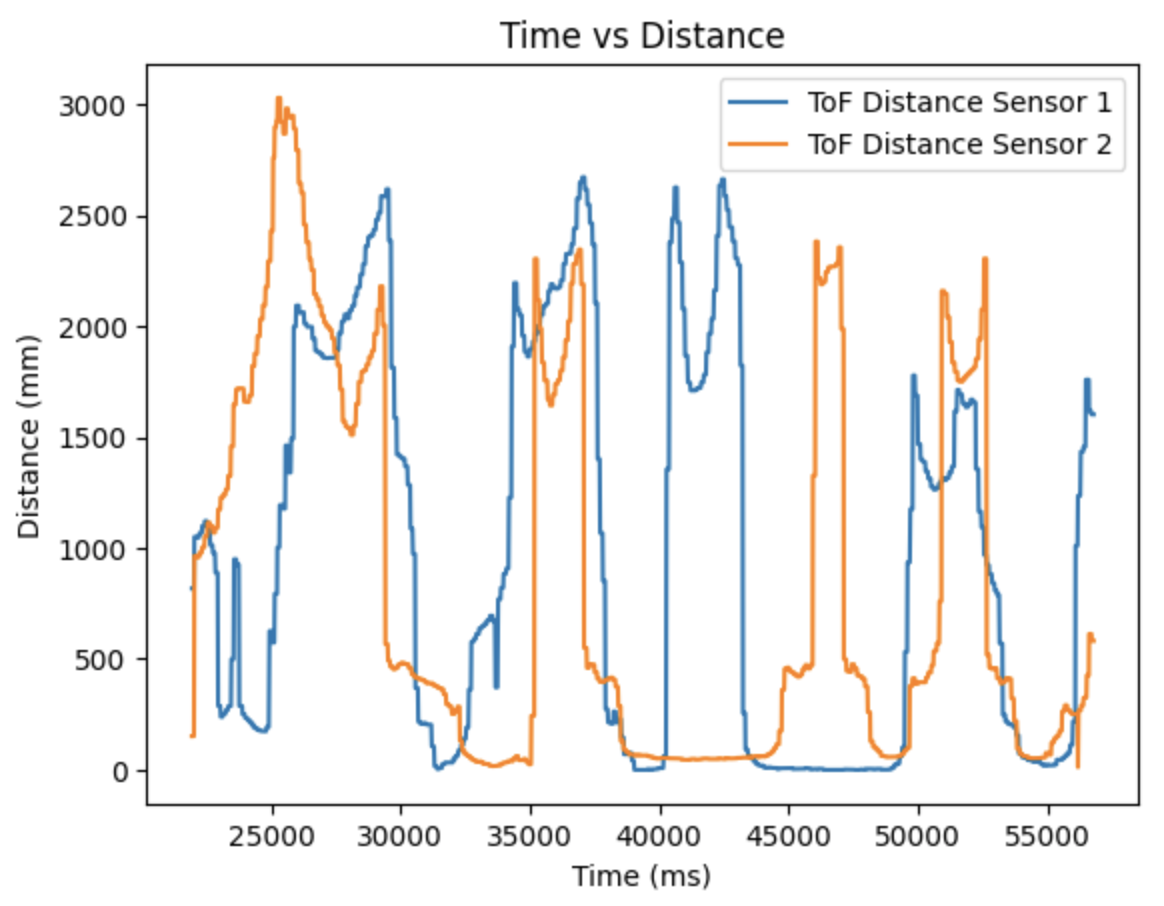
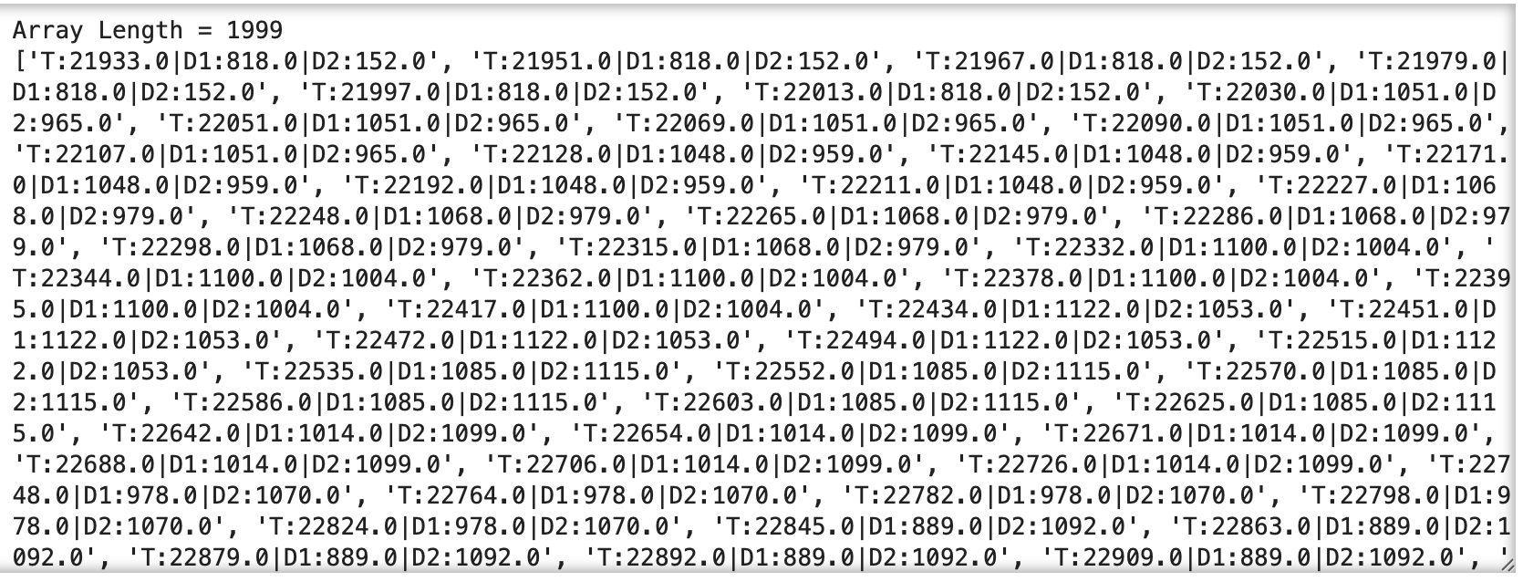
Time vs Distance: Data From Two ToF Sensors Over Bluetooth
The code from Lab 2 was modified to send time stamped ToF sensor data to Jupyter Notebook. The data for the two ToF sensors was plotted against the recorded time.
Lab 2: IMU
The objective of the lab is to connect the IMU to the Artemis board and record the robot performing a stunt.
Lab Tasks
Artemis IMU Connections
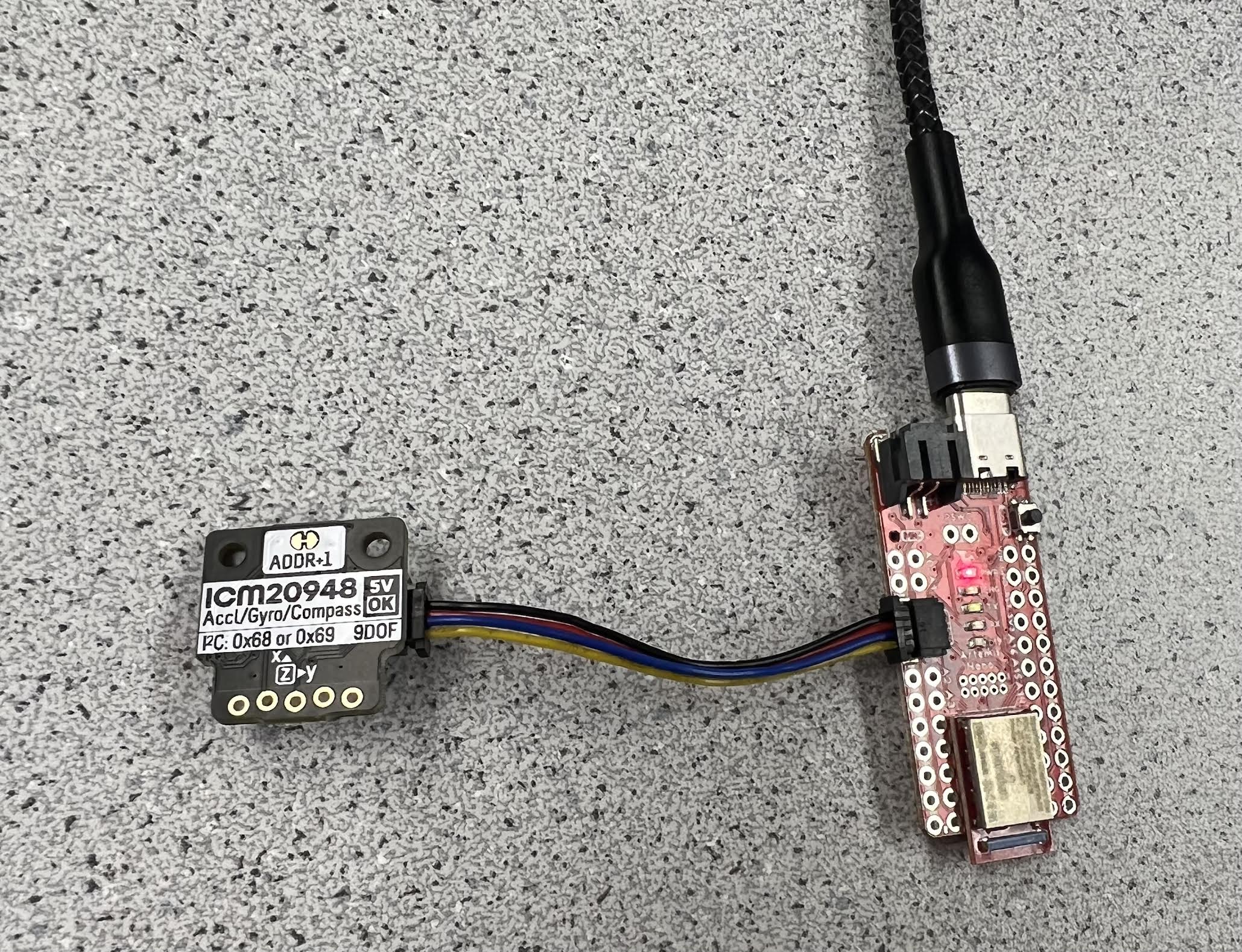
The setup for this lab is shown in the image below.
IMU Example Code and AD0_VAL
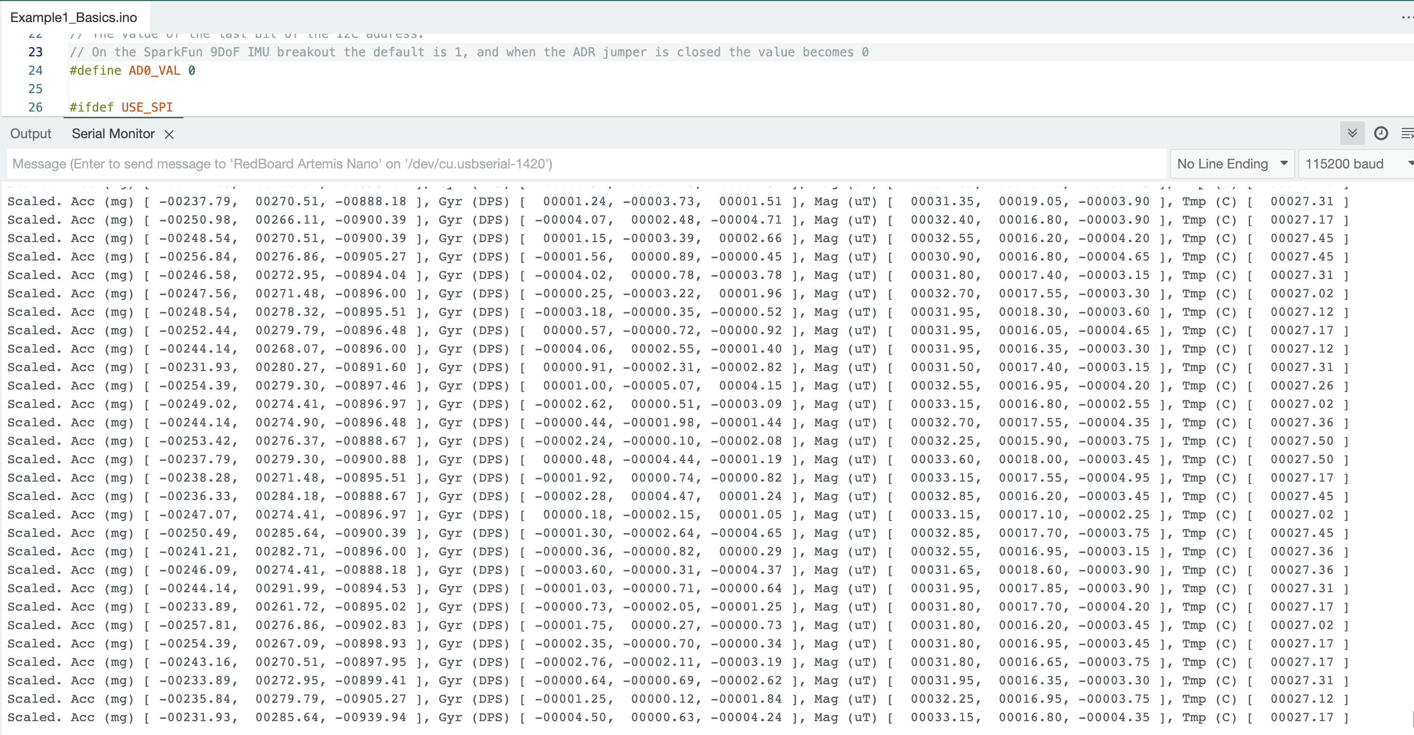
The example code found under SparkFun 9DOF IMU Breakout - ICM 20948 - Arduino Library->Arduino->Example1_Basics was run to test if the IMU was working correctly.
Upon opening the Example1_Basics code, the AD0_VAL default was set to one. When the ADR jumper is closed the value should be set to zero. AD0_VAL corresponds to the last bit of the I2C address. My ADR jumer on the IMU was closed. For this reason, I needed to change the AD0_VAL to zero to return the accelerometer, gyroscope, magnetometer, and temperature data.
While viewing the output data in the serial monitor, I moved the IMU to change the accelerometer and gyroscope data. I looked at the notated axis that was printed on the IMU and moved the IMU along the X, Y, and Z axis. I noticed that the respective X, Y, and Z serial monitor outputs for the accelerometer increased when I moved the IMU along the respective positive axis. The gyroscope data for pitch, roll, and yaw also changed when I rotated the IMU around the X, Y, and Z axis.
Adding A Slow Blink
In the Example1_Basics code, I added a slow blink at the beginning of void setup() to turn the Artemis LED on and off three times.
Accelerometer
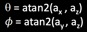
Accelerometer Equations
The following equations for pitch (theta) and roll (phi) were found in the FastRobots-4-IMU Lecture Presentation.
Accelerometer Pitch and Roll at -90, 0, and 90 degrees
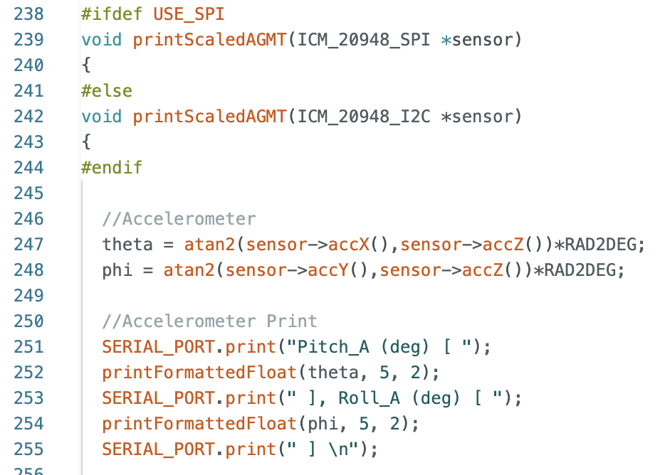
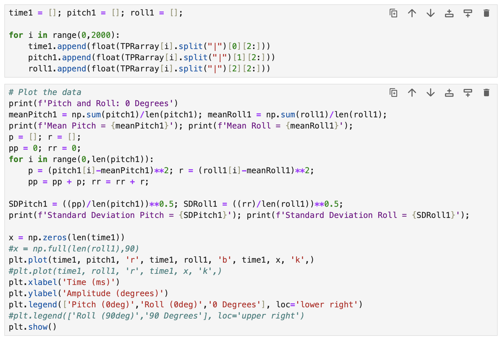
These equations were used to compute pitch and roll for the accelerometer. I implemented the calculations in the Example1_Basics sketch (lines 247 - 255 below) that was used in the previous task to receive continuous data from the Artemis board and plot the results.
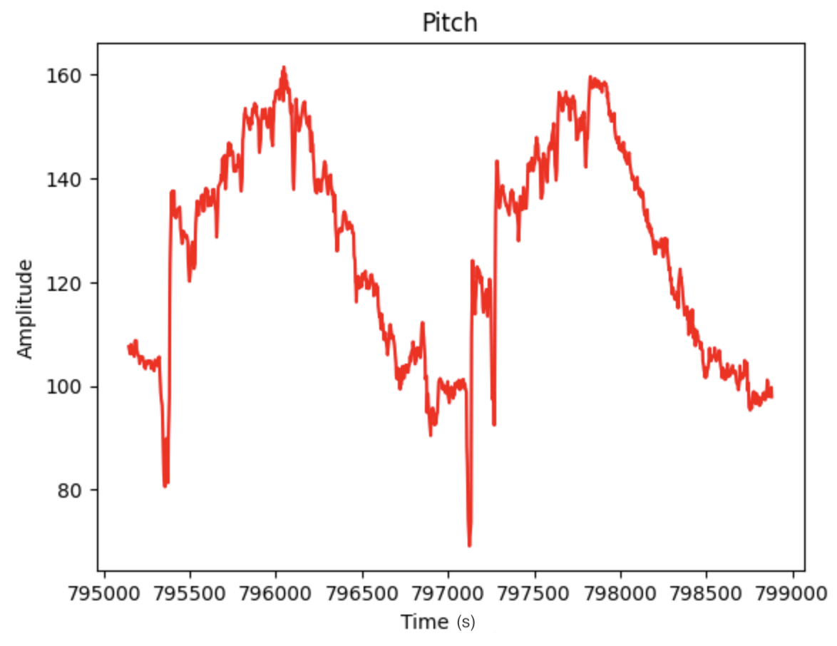
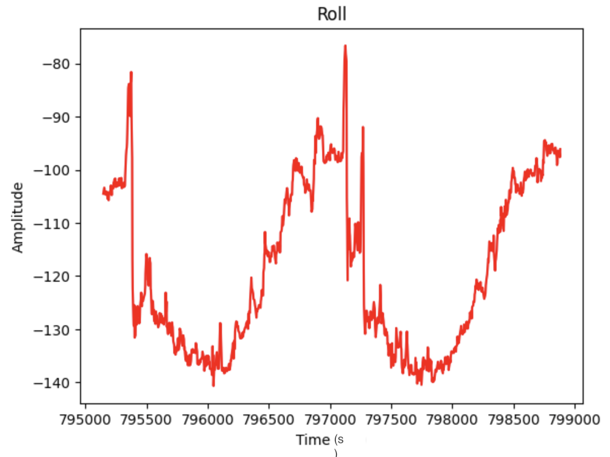
The below graphs show Pitch (data 0, green) and Roll (data 1, purple) at 0 degrees. The x-axis is time (sec) and the y-axis is degrees.
Pitch and Roll at 0 degrees:
.png)
The below graphs show Pitch (data 0, green) at -90 and 90 degrees and the corresponding Roll (data 1, purple) outputs. The x-axis is time (sec) and the y-axis is degrees. From the graphs it can be seen that when pitch is at -90 degrees there is noise in the roll outputs.
Pitch at -90 degrees:
.png)
Pitch at 90 degrees:
.png)
The below graphs show Roll (data 1, purple) at -90 and 90 degrees and the corresponding Pitch (data 0, green) outputs. The x-axis is time (sec) and the y-axis is degrees.
Roll at -90 degrees:
.png)
Roll at 90 degrees:
.png)
Accuracy Analysis
I plotted the data for pitch and roll at 0, 90, and -90 degrees in Jupyter Notebook and calculated the mean and standard deviation.
Below are graphs. I also included a black line at 0, 90, or -90 degrees for reference. Note: The data for the graphs was collected by holding the IMU against the table using my hand. This may have resulted in some error due to the surface level or any small hand movements. In the future the IMU should be calibrated when it is secured to the robot to achieve the most accurate pitch and roll data.
Analysis.png)
.png)
.png)
.png)
.png)
Fast Fourier Transform (FFT) Graphs
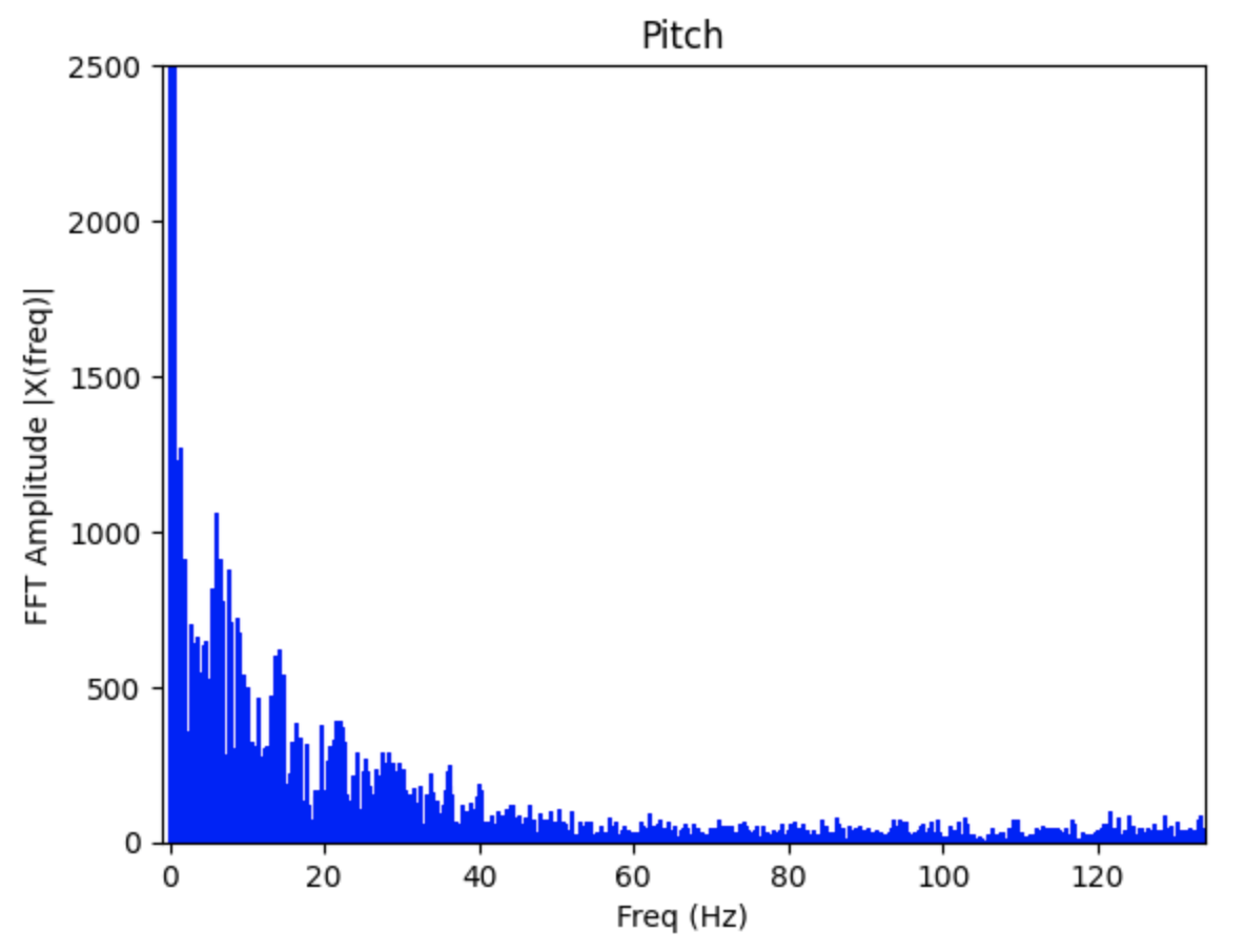
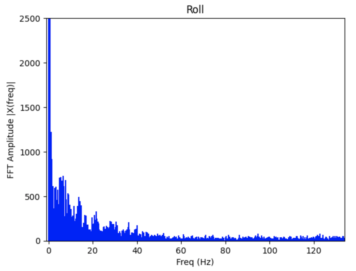
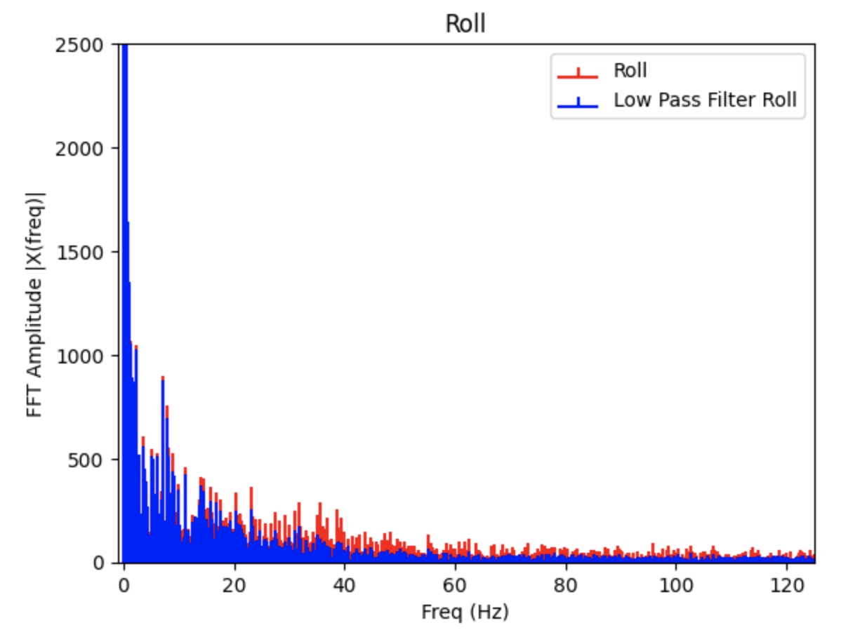
The noise in the accelerometer was examined using a Fast Fourier Transform. Data for the FFT was collected as I moved the IMU. The sinusoid and the FFT graphs can be found below. There is a large spike closer to 0Hz and less noise as the frequency increases. Note: I modified the code from Stephan Wagner's Ed Discussion post to plot the FFT graphs.
Low Pass Filter FFT Graphs
From observing the above graphs, I choose a cutoff frequency of 25Hz to use for a low pass filter. Using the determined cutoff frequency, I calculated the alpha used in the low pass filter. The equations from lecture are below:
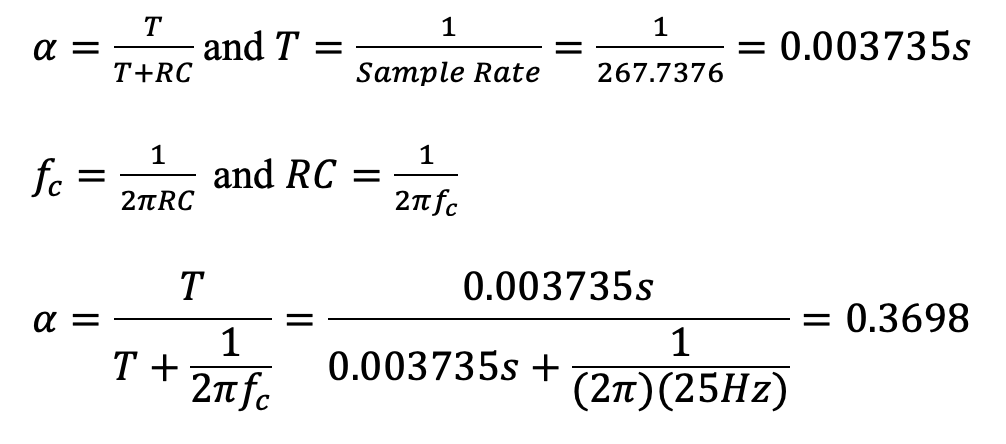
The low pass filter alpha was calculated to be 0.3698
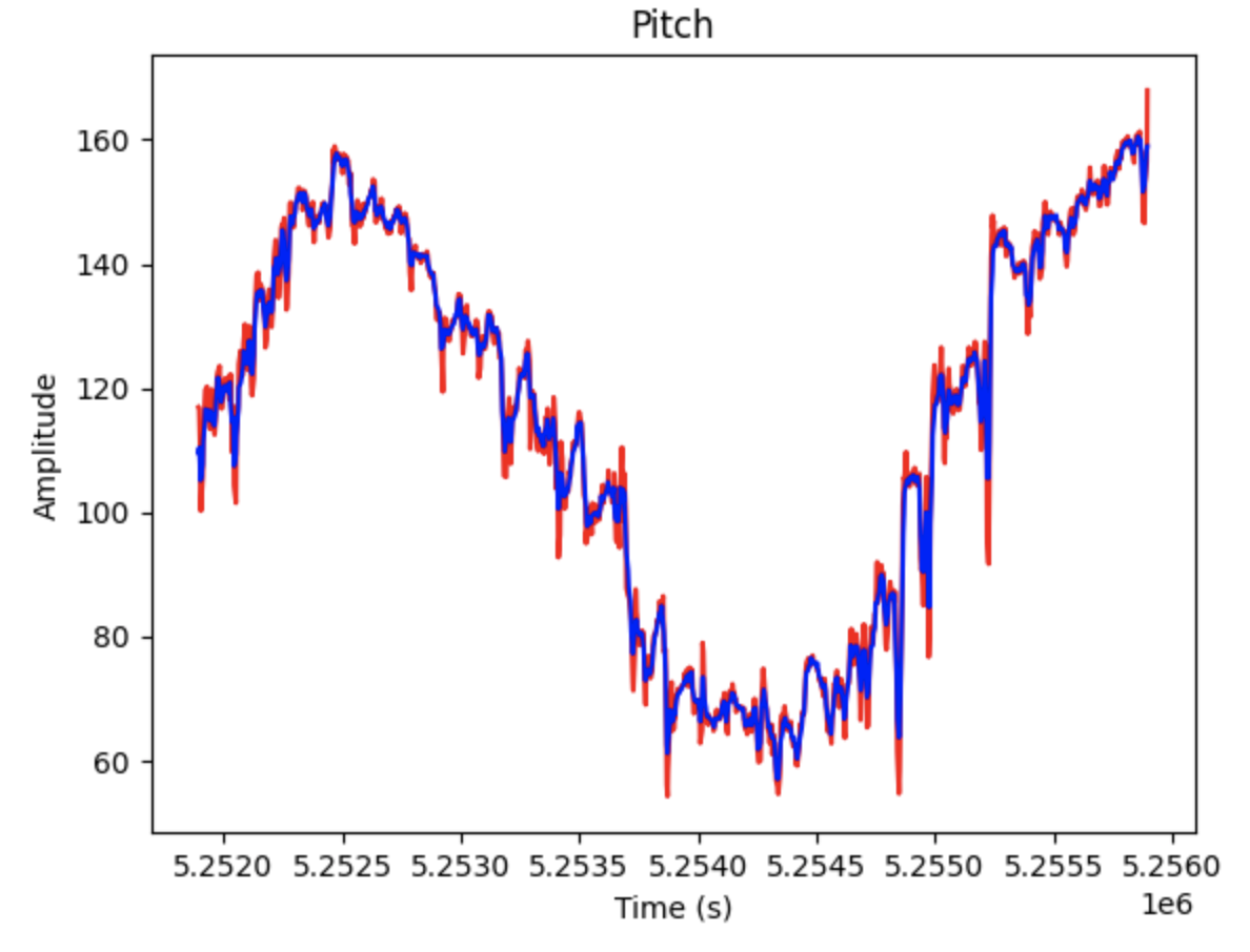
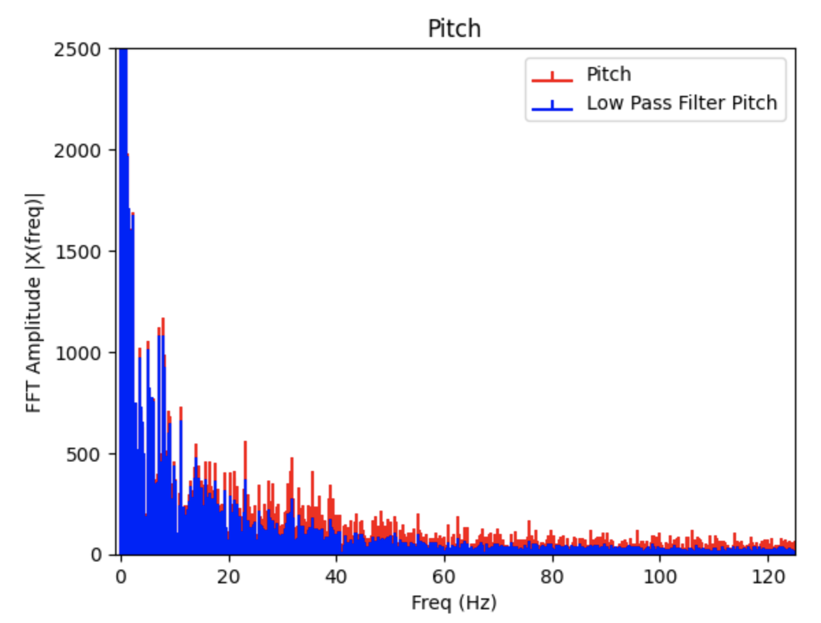
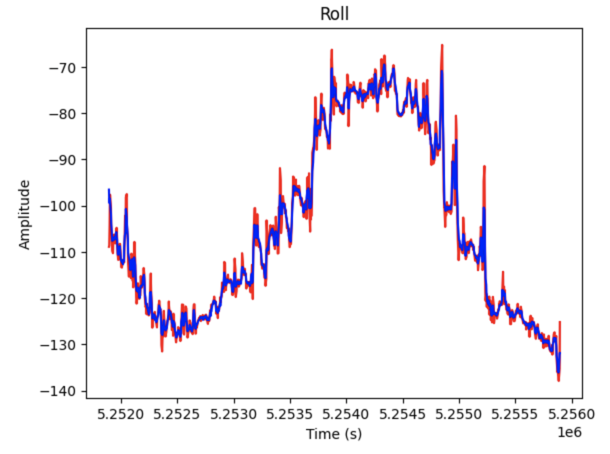
The below FFT graphs show the original signal (red) and the reduction in noise after implementing a low pass filter (blue). Choosing a lower cut off frequency reduces more noise.
Gyroscope
Gyroscope Equations
The following equations for pitch, roll, and yaw were found in the FastRobots-4-IMU Lecture Presentation.

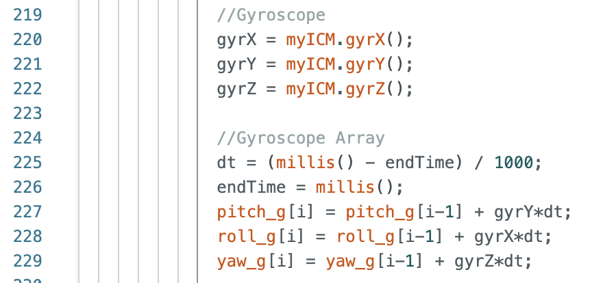
The gyroscope measures angular velocity. To find pitch, roll, and yaw the data collected from the IMU needs to be multiplied by a time step (dt in the below code).
Gyroscope vs. Accelerometer Outputs
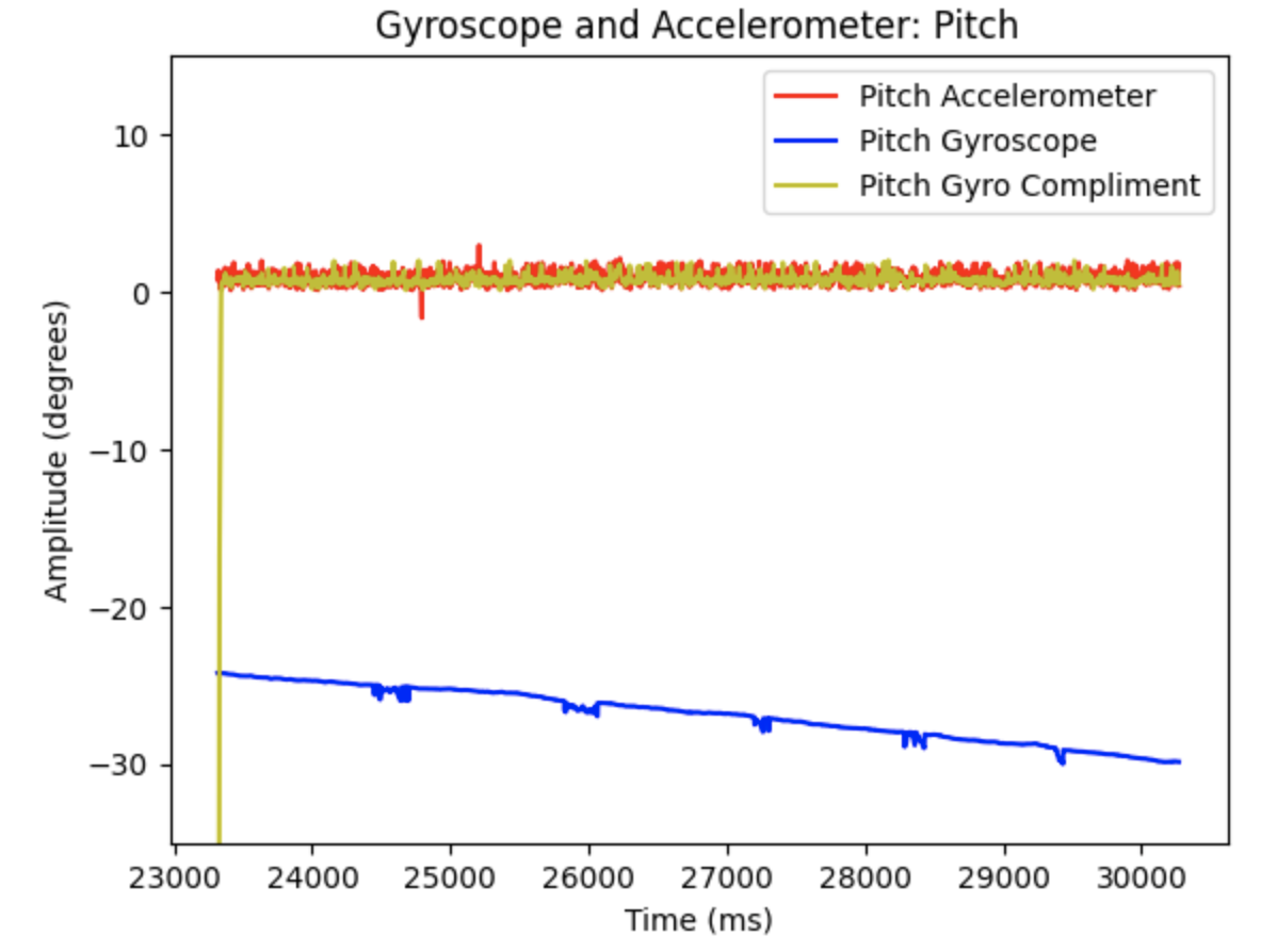
The code above was added to Example1_Basics and plotted alongside the data for the accelerometer's pitch and roll. The gyroscope data drifts over time, but has less noise then the accelerometer data. In the below graphs the IMU was moved slightly to achieve different outputs.
Pitch for Gyroscope (Blue) and Accelerometer (Orange):
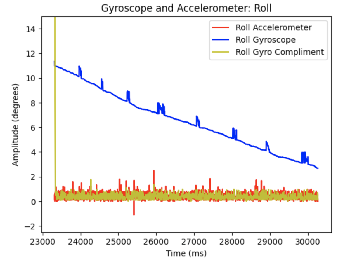
Roll for Gyroscope (Blue) and Accelerometer (Teal):
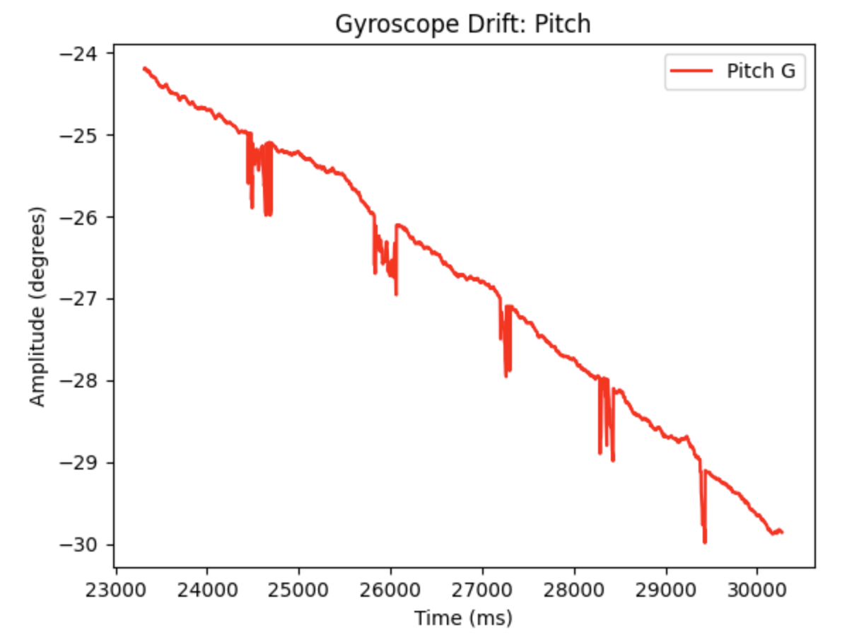
The drift for the gyroscope can be better seen in the below graphs. The gyroscope was held in the same position as the data was collected. As time increases the measurements drift away from the starting value.
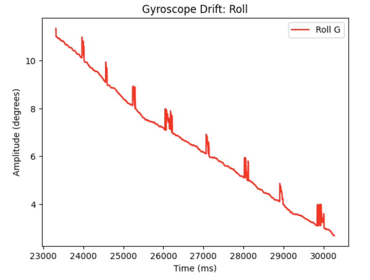
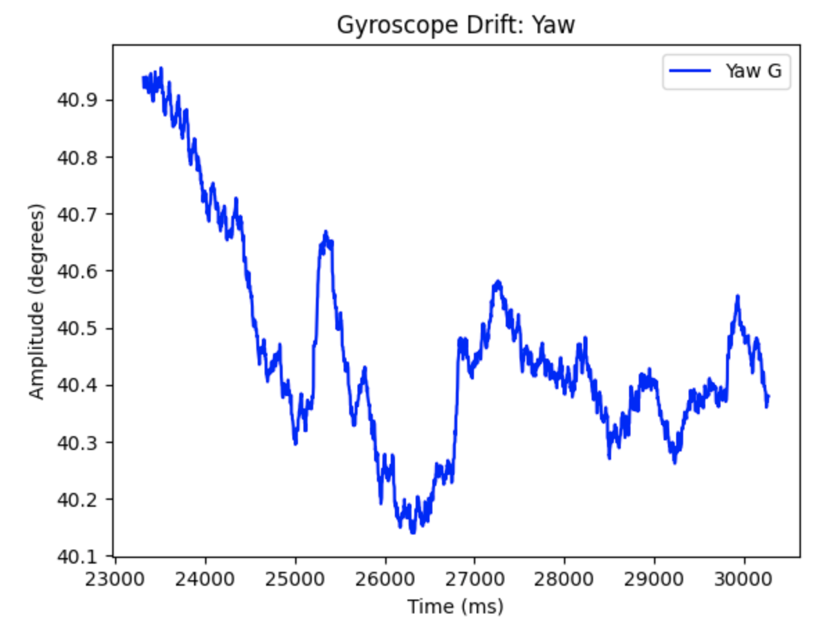
Code to plot the above graphs:
Adjusting The Sampling Frequency
Decreasing the sampling frequency resulted in a slower update to the angle measurements and more variation in the outputs between each successive measurement. The sample rate should be high to achieve the greatest level of accuracy when recording data.
Complimentary Filter
Complimentary filter equation from lecture:

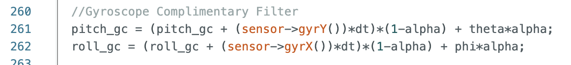
The complimentary filter shows resistance to small vibrations as the IMU is moved during data collection. The complimentary filter reduces noise compared to the accelerometer output. Alpha is a set constant that represents how well the accelerometer output measures the correct pitch and roll data. I examined how different alpha values affected the graphs. In the below graphs alpha = 0.5
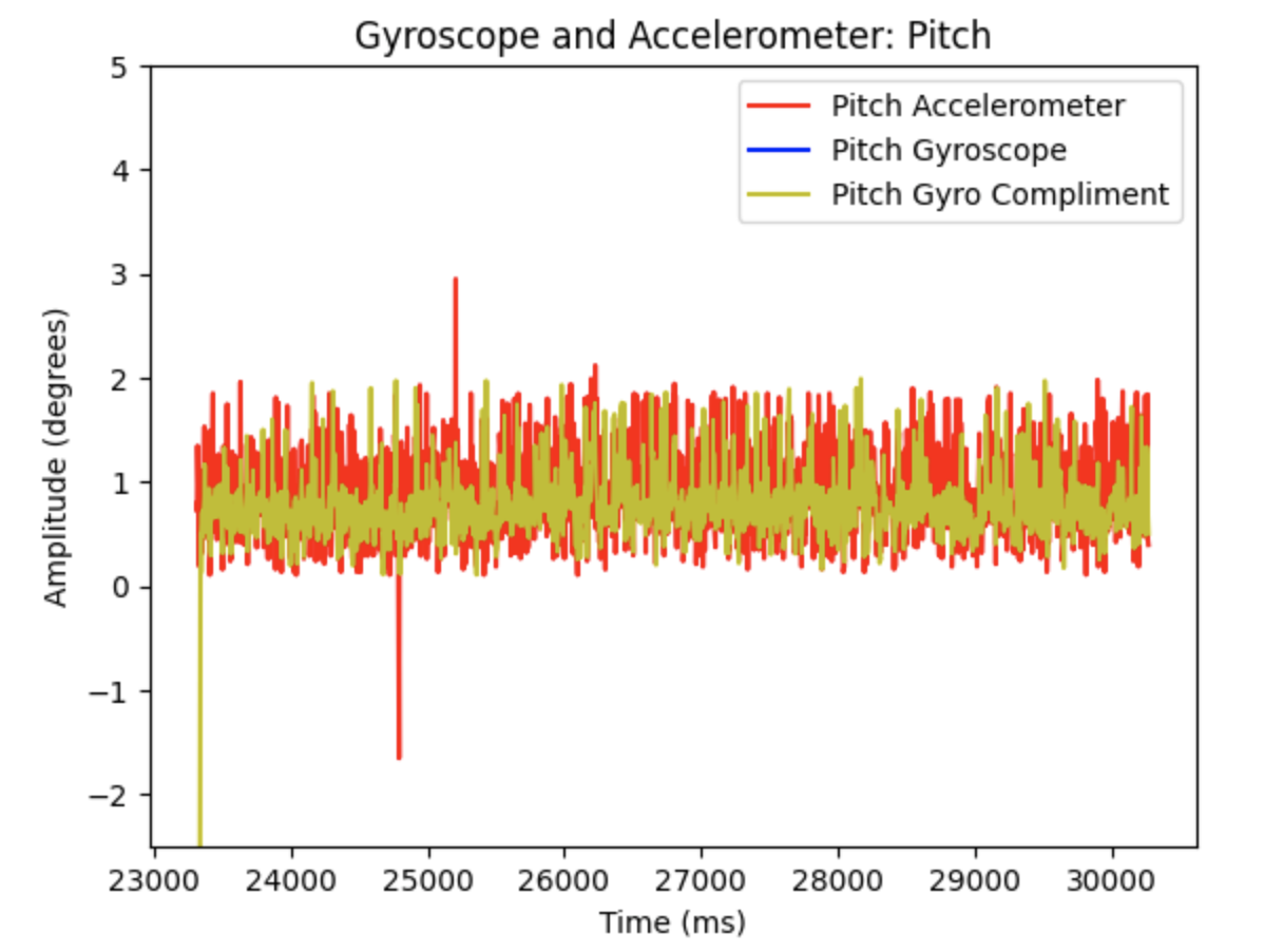
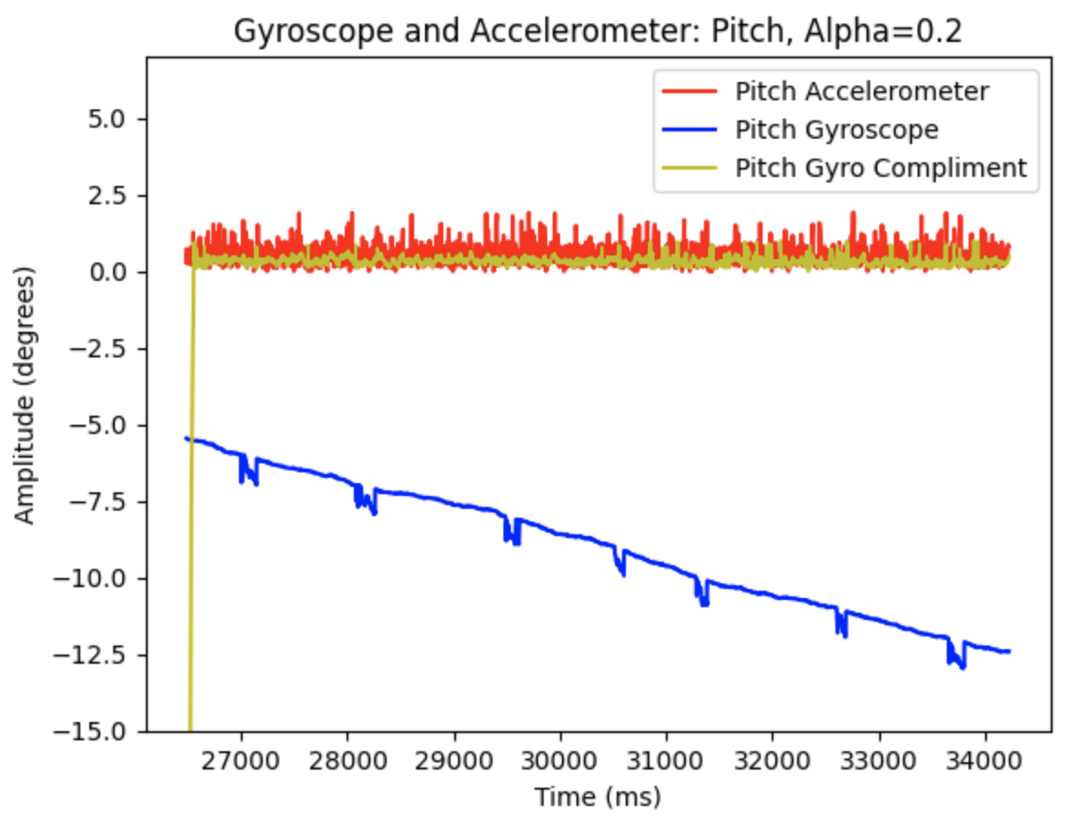
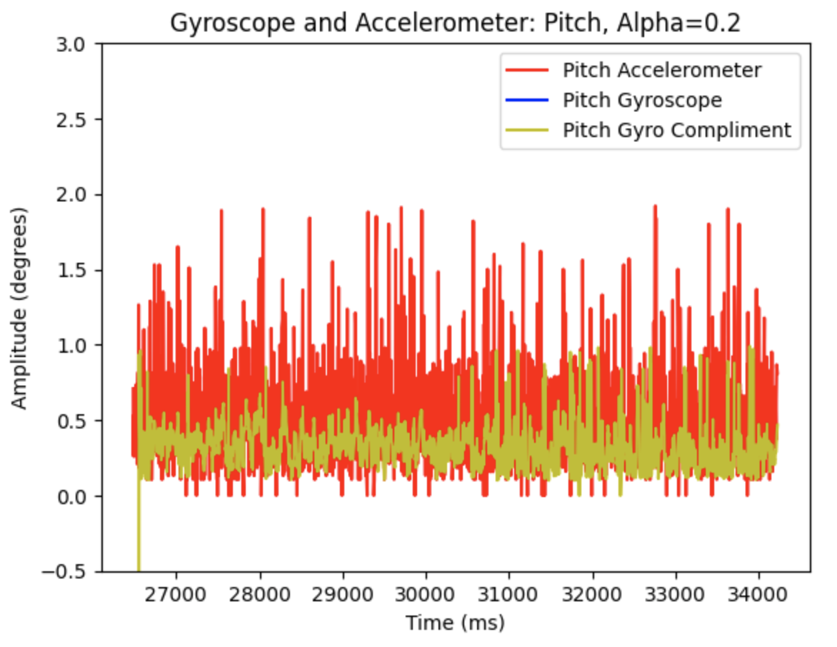
Pitch for Gyroscope (Blue), Gyroscope Complimentary Filter (Orange), and Accelerometer (Teal):
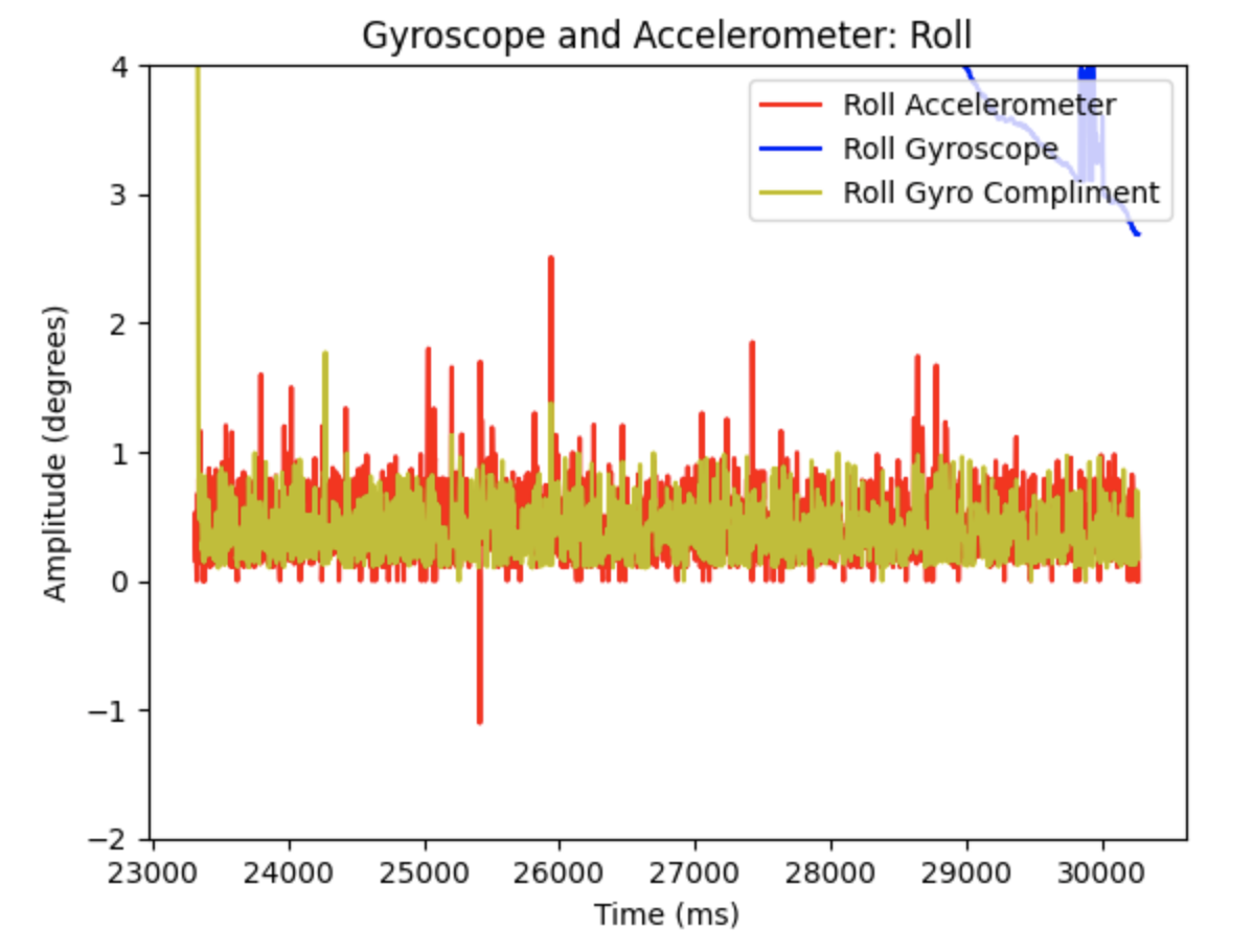
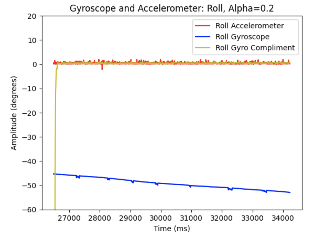
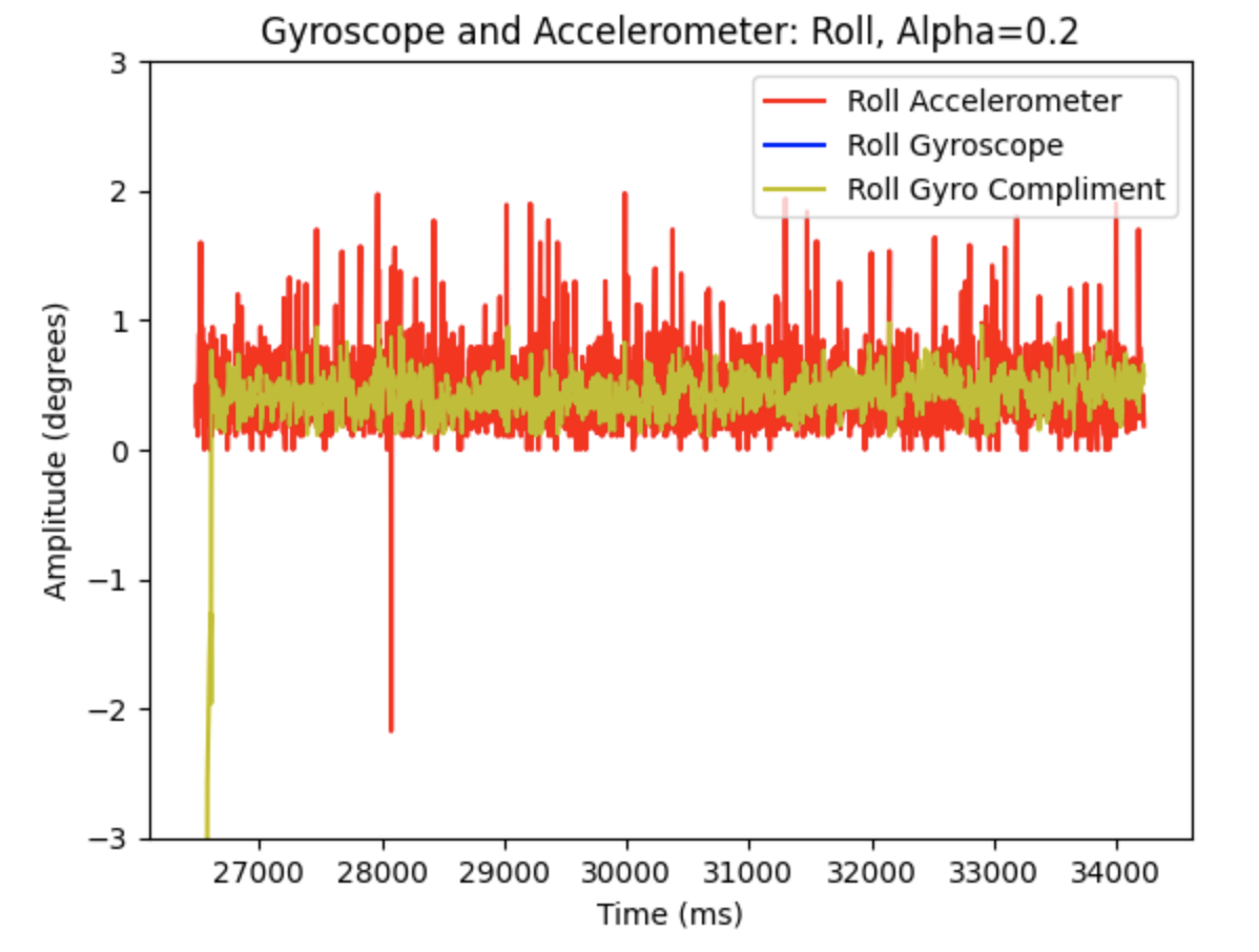
Roll for Gyroscope (Blue), Gyroscope Complimentary Filter (Orange), and Accelerometer (Teal):
Pitch for Gyroscope, Gyroscope Complimentary Filter, and Accelerometer (alpha = 0.5):
Roll for Gyroscope, Gyroscope Complimentary Filter, and Accelerometer (alpha = 0.5):
Additional graphs when alpha = 0.2
Code to plot the above graphs:

Sample Data
Speed Of Sampling
All of the accelerometer and gyroscope data print statements and any delays in the ble_arduino.ino file were removed in order to speed up the execution of the main loop. A case called "ACC_GYR" was created that checked if the data was ready in the main loop, and if there was data available stored it in arrays. After speeding up the loop I found that new values were sampled every 0.04s, which is a sampling frequency of 1/0.04s = 25Hz.
Collect And Store Time Stamped IMU Data In Arrays
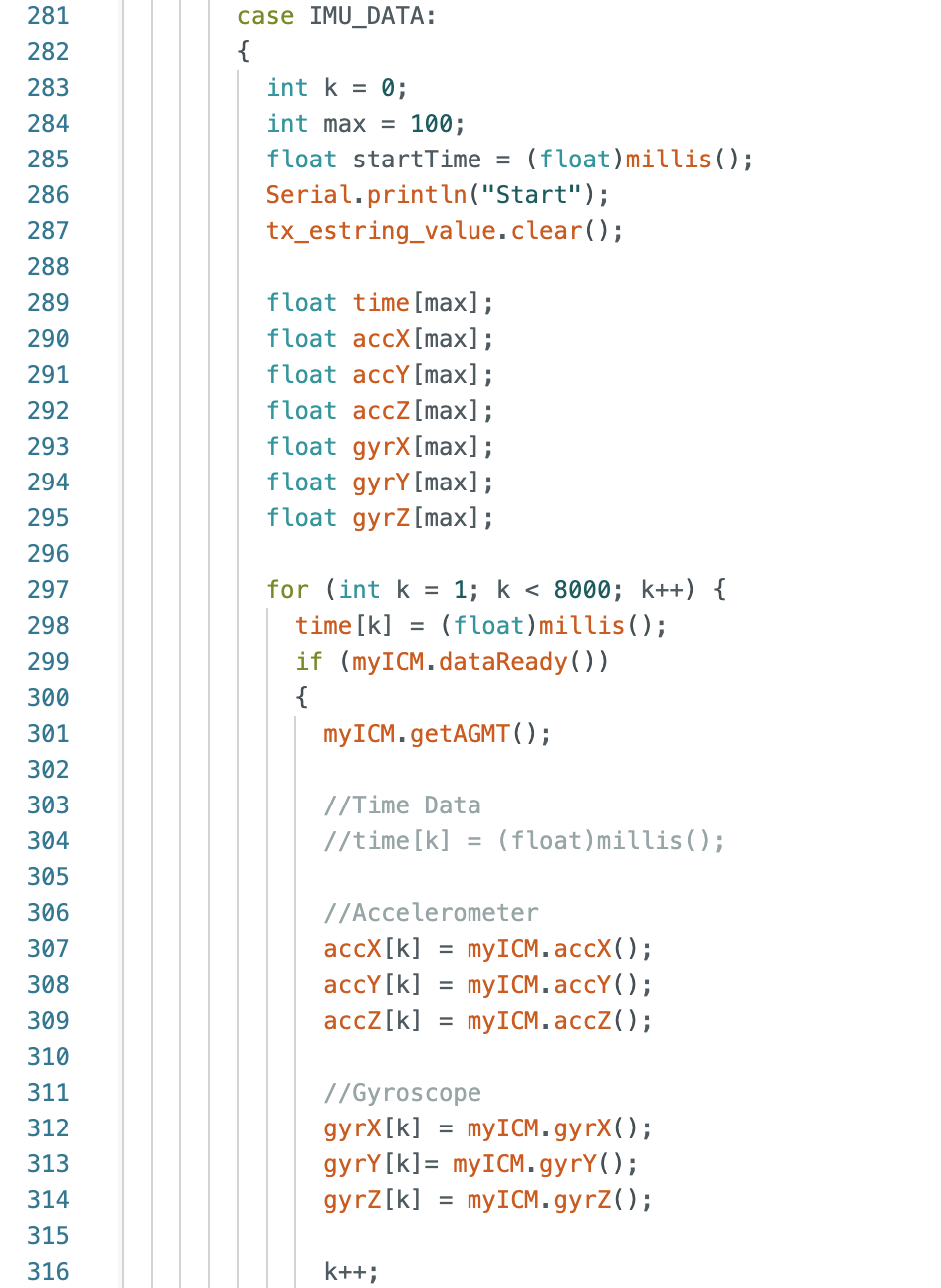
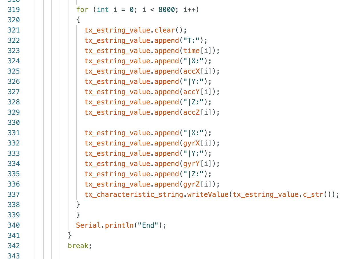
The data is stored in arrays on the Artemis board before being sent to Jupyter Notebook. There are 7 arrays including time (1); accelerometer: x (2), y (3), z (4); gyroscope: x (5), y (6), z (7). I choose to use separate arrays because in the future I can decide what data I want to send to Jupyter Notebook. The data type used to store the data is a float. I choose to use a float as it is less bytes then a double, allowing for more data to be stored on the memory of the Artemis. A float is 4 bytes, resulting in one packet of data information for the 7 arrays to be 28 bytes. The Artemis has 384kB of RAM. Sampling at 0.04s (25Hz) will result in data being collected for 548 seconds.
Code to find X, Y, and Z for Accelerometer and Gyroscope.
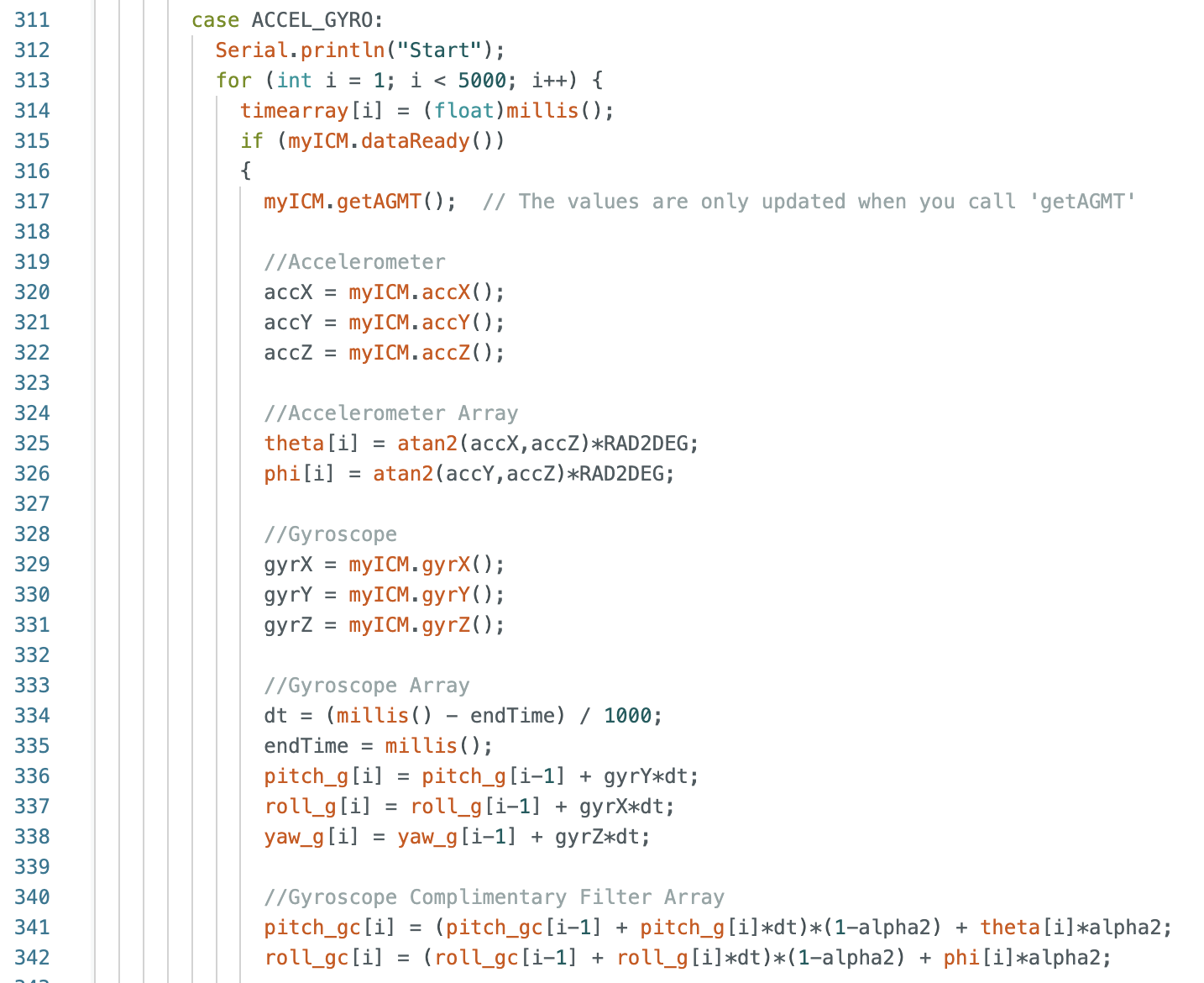
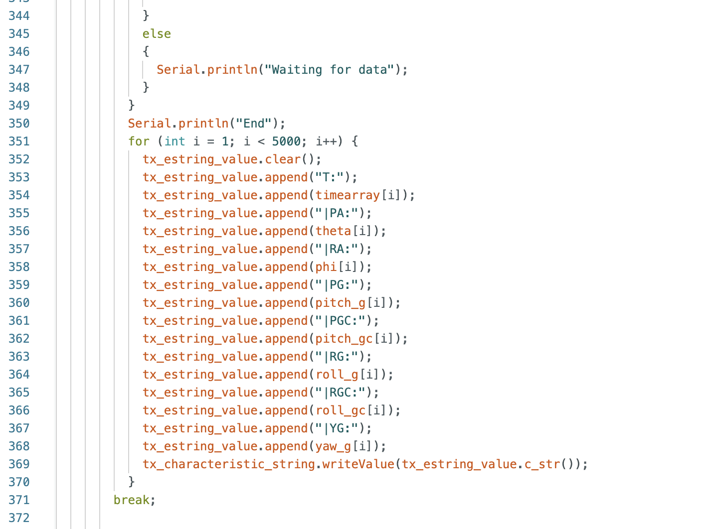
Code to find pitch and roll for Accelerometer; and pitch, pitch compliment, roll, roll compliment, and yaw for Gyroscope.
Lab 1: The Artemis Board and Bluetooth
Part 1
Test the connection between the Artemis board and the computer. Arduino IDE was installed and a number of tasks were completed to show the functionality of the Artemis board.
Lab Tasks
Tasks 1 and 2: "Example: Blink It Up"
The instructions for Arduino Installation were followed to ensure proper connection between the Artemis board and the computer. The SparkFun Apollo3 Boards package was installed using the Boards Manager in Arduino IDE (shown below).

The first task involved a blinking LED on the Artemis board. Example code: File->Examples->01.Basics->Blink. A loop was implemented and used the function digitalWrite() to turn on the LED for one second and then turn off the LED for one second (shown below).
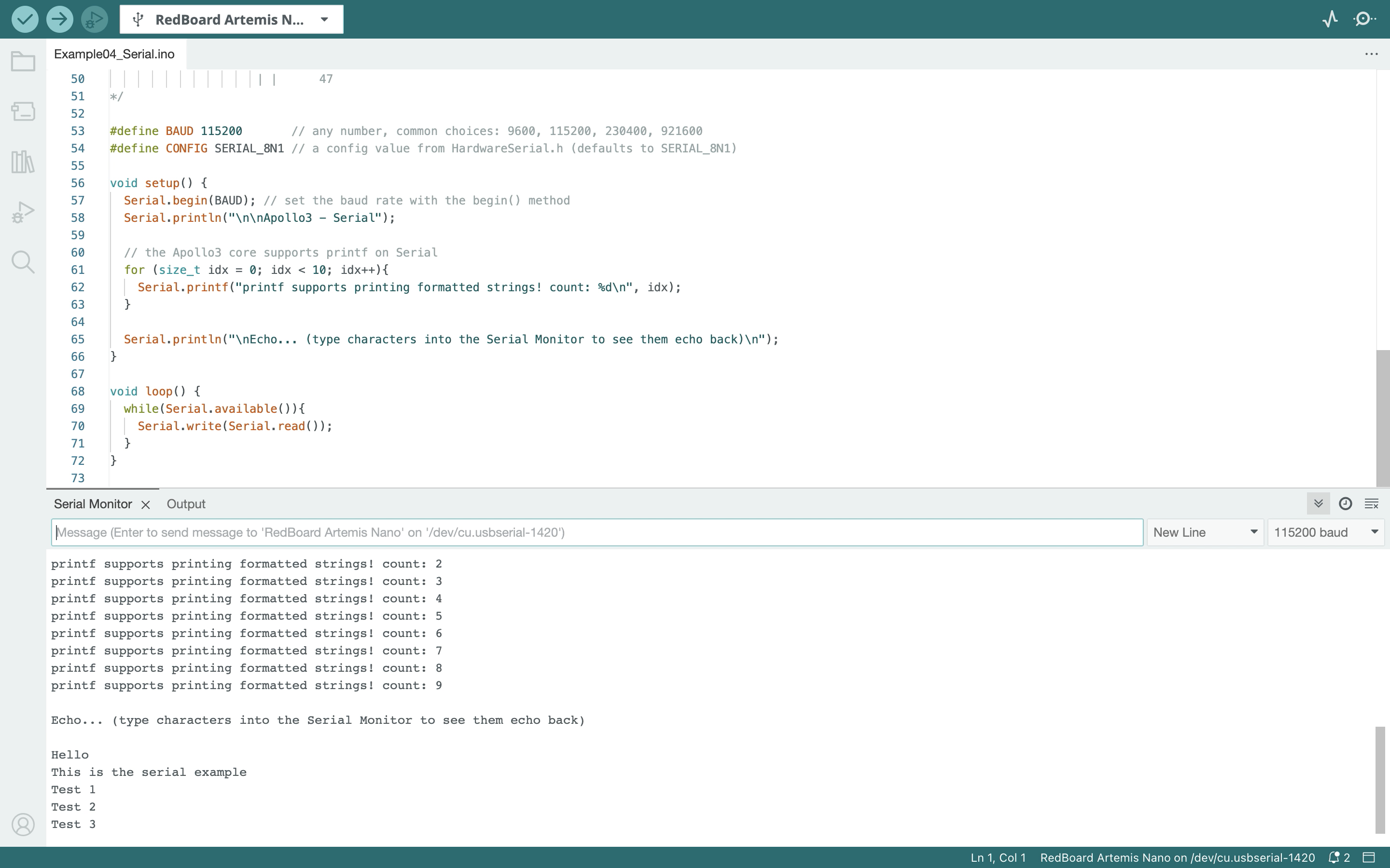
Task 3: Example04_Serial
In this example serial communication between the Artemis board and the computer was tested. Example code: File->Examples->Apollo3->Example04_Serial.
Below is an image and video of the Serial Monitor showing the outputs: "Hello", "This is the serial example", "Test 1", "Test 2", and "Test 3".
Task 4: Example02_AnalogRead
The temperature sensor of the Artemis board was tested. Example code: File->Examples->Apollo3->Example02_AnalogRead. I covered the sensor with my hand to increase the temperature reading. At the beginning of the test the temperature is around 32.3 degrees Celsius and reaches a temperature of around 33.4 degrees Celsius (shown below).
Another example shows various temperatures being plotted using Better Serial Plotter.

Task 5: Example1_MicrophoneOutput
The Microphone Output task tests the microphone of the Artemis board. Example code: File->Examples->PDM->Example1_MicrophoneOutput. During this task I spoke into the microphone to change the frequency (image and video shown below).
5000 Level Task 1: LED and Musical A4
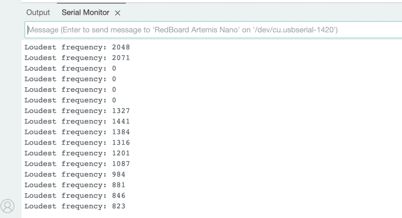
The Artemis board was programmed to turn on the LED when the musical note A4 is played on a speaker (code below). I started with the Example01_MicrophoneOutput sketch, and I added if statements (lines 113-122 below). The note A4 is 440Hz (UC Berkeley Reference). The first if statement determines if the frequency is between 430Hz and 450Hz to account for any slight error in sound quality. If the frequency is within range an “A4” statement will be displayed in the Serial Monitor and the LED on the Artemis board will turn on. The second if statement determines if the frequency is lower than 430Hz or greater than 450Hz. If the frequency is lower than 430Hz or greater than 450Hz a “Not A4” statement will be displayed in the Serial Monitor and the LED on the Artemis board will turn off.
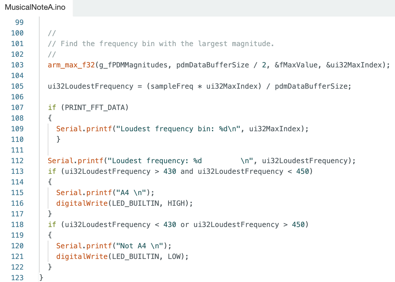
Image of the outputs in the serial monitor:

Video showing the LED turning on when the note A4 is played:
I added to the LED and Musical A4 task by creating a musical tuner. There are eleven total if statements that determine the note being played (lines 113-168 below):


Video of various notes being played:
Discussion: Part 1
I tested the connection between the Artemis board and the computer. Tasks performed included turning on and off an Artemis board LED, printing serial monitor outputs, viewing temperature data in the serial monitor, testing the microphone, and creating a musical tuner.
Part 2
Tested the Bluetooth communication between the computer and the Artemis board. Python in a Jupyter Notebook was used for the computer and Arduino IDE was used for the Artemis board.
Prelab: Setup
During the setup for the lab I already had installed Python 3. I needed to install pip by running the line "python3 -m pip install --user virtualenv" in the Command Line Interface (CLI). I created a folder called “MAE 5190 Lab” where I put all of the Jupyter Notebook files. I then created a virtual environment by typing "python3 -m venv FastRobots_ble" in the CLI.
The virtual environment was activated by typing "source FastRobots_ble/bin/activate" and then deactivated by typing "deactivate".
The python packages were installed by entering "pip install numpy pyyaml colorama nest_asyncio bleak jupyterlab" into the CLI.
CLI entered commands:


I also needed to install matplotlib to use for the 5000 level tasks. I asked a TA for help with the installation. Below is a picture of the command entered into the CLI.
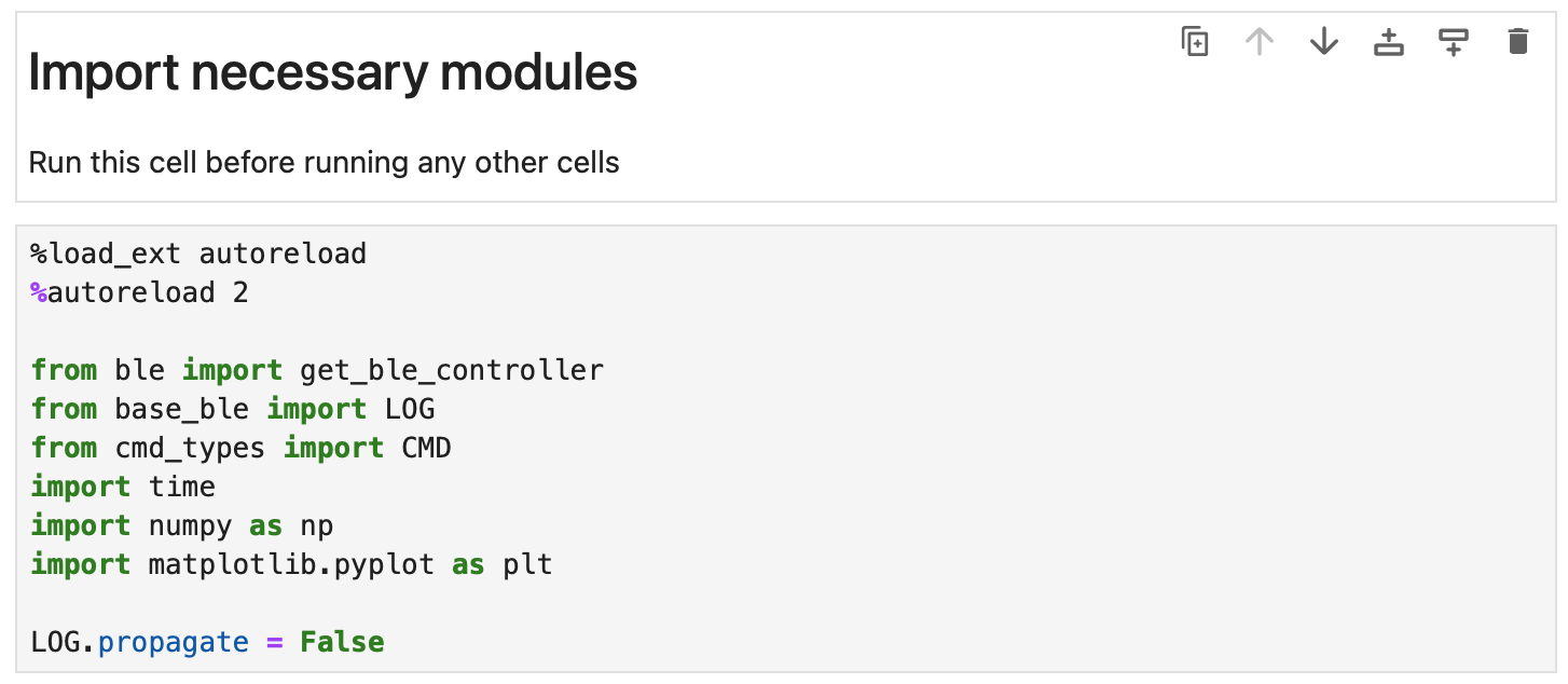
To import modules into the Jupyter Notebook the following lines of code were run.
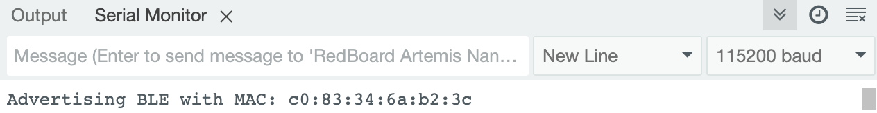
After uploading the provided ble_ardunio.ino file to the Artemis board the MAC address was printed in the serial monitor. The MAC address is c0:83:34:6a:b2:3c The image below shows the Arduino serial monitor with the printed MAC address.
Prelab: Codebase
I installed the provided codebase into the project directory and copied the provided “ble_python” directory into the project directory. Then the Jupyter Notebook was opened by entering “jupyter lab” into the CLI (shown below).
To set up Bluetooth communication, the MAC address needed to be changed in the Jupyter Notebook connection.yaml file to match the advertised MAC address from the Artemis board. Then unique UUID addresses needed to be used in the connection.yaml file and Arduino IDE because some devices in the lab may have the same MAC address. Using UUIDs ensures that the computer is receiving data from the correct Artemis board. The UUIDs were generated in the Jupyter Notebook demo.ipynb file and then entered into the connection.yaml and ble_arduino.ino files. Below is a picture of the lines of code used in the demo.ipynb file to generate the UUIDs.

The UUIDs were entered into the ble_arduino.ino file:

The UUIDs were entered into the connection.yaml file:

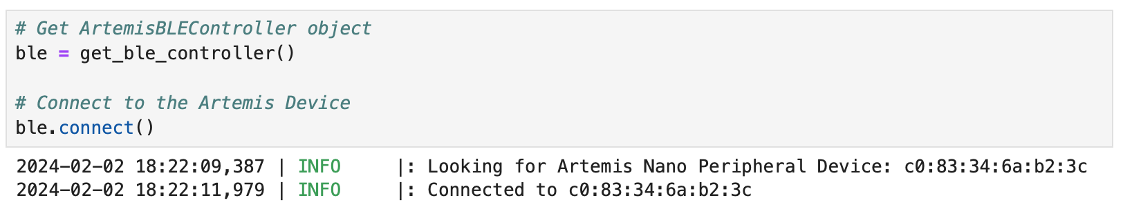
To connect to the Artemis the following lines were run in the Jupyter Notebook.
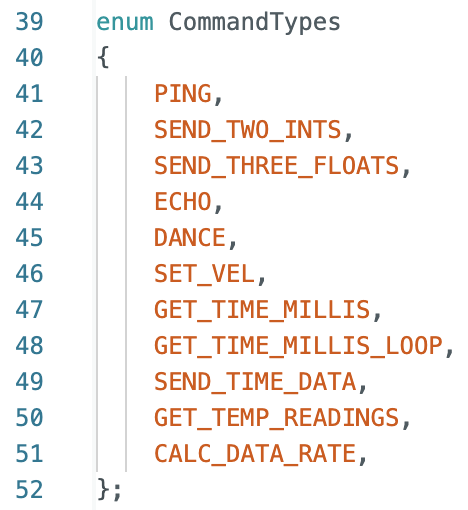
Several command types needed to be defined to complete the tasks outlined in the next section. Added commands include ECHO, GET_TIME_MILLIS, GET_TIME_MILLIS_LOOP, SEND_TIME_DATA, and GET_TEMP_READINGS.
Command types defined in Arduino IDE:
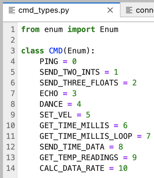
Command types defined in Jupyter Notebook:
Lab Tasks
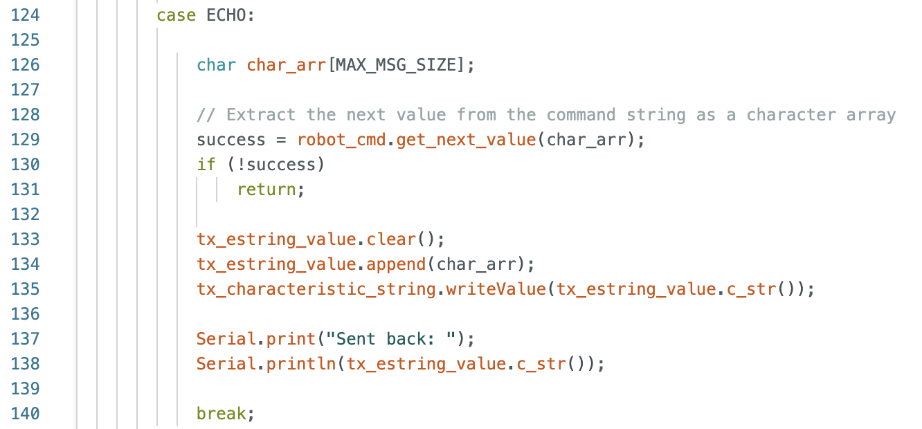
Task 1: ECHO Command
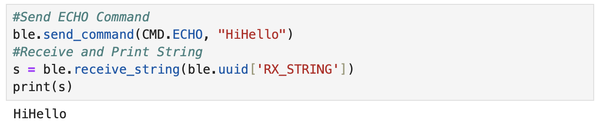
The first task was to send an ECHO command of a string value to the Artemis board and receive an augmented string on the host computer. This task tested the communication between the Artemis board and the computer.
The image below shows the Arduino IDE code.
Jupyter Notebook code to send the ECHO command and receive the augmented string from the Artemis board:
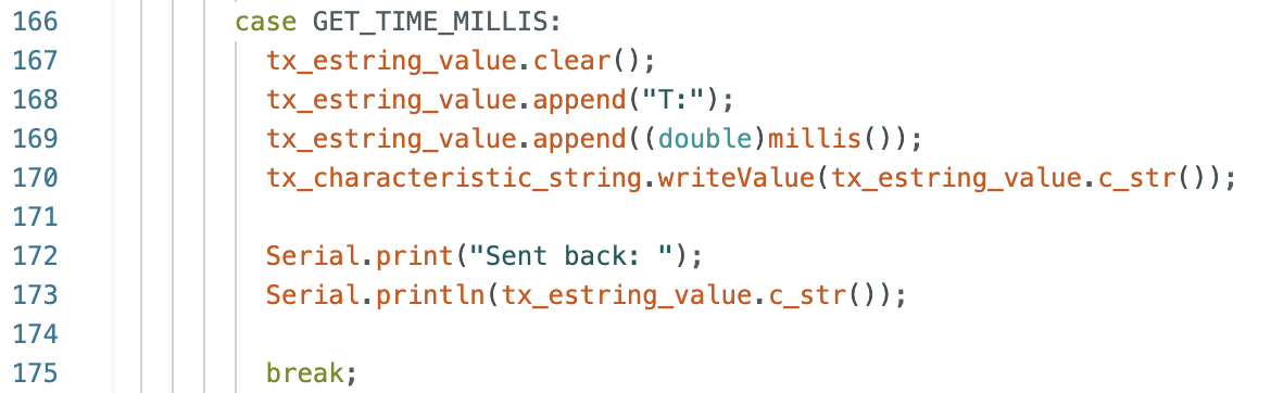
Task 2: GET_TIME_MILLIS
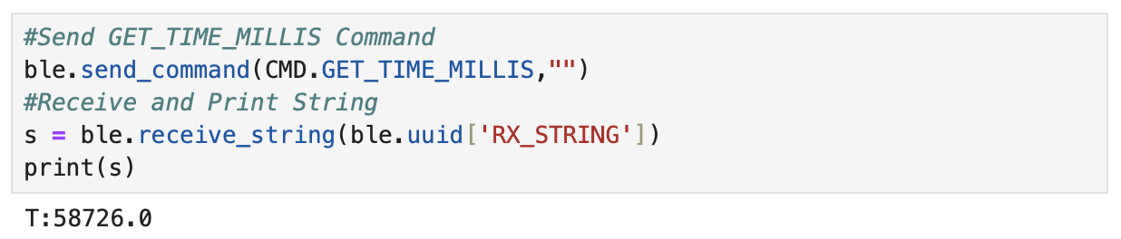
The next task adds another command to the Jupyter Notebook for the Artemis board to reply with a string of the current time.
The image below shows the Arduino IDE code.
Jupyter Notebook code to send the GET_TIME_MILLIS command and receive the string with the current time:
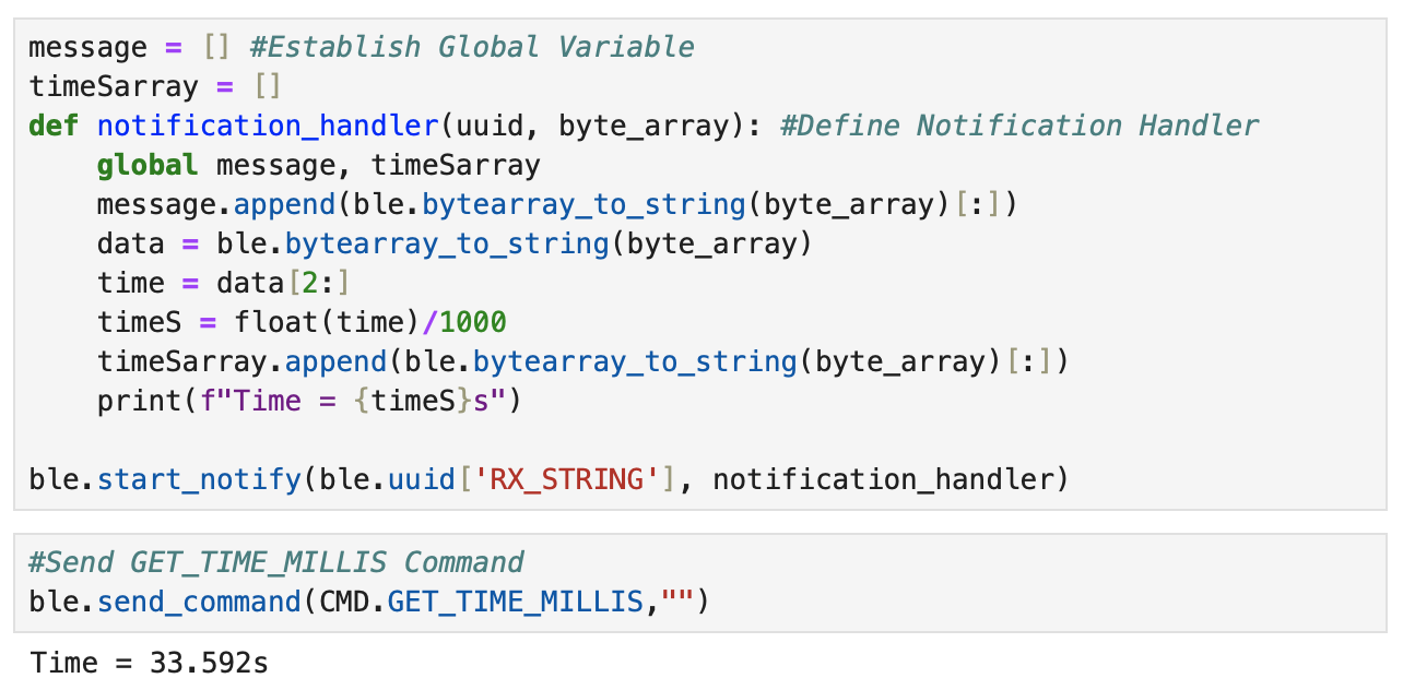
Task 3: Notification Handler
A notification handler was created in the Python Jupyter Notebook to receive a string value from the Artemis board. The GET_TIME_MILLIS command was used to get the time after starting the notification handler.
The image below is the notification handler and the GET_TIME_MILLIS command in the Jupyter Notebook.
Task 4: Current Time Loop
A loop was implemented to get the current time in milliseconds from the Artemis board and send the information to the computer. The time information is received and processed by the notification handler.
To find the data transfer rate the length of the data was computed by assembling the individual outputs into an array in the Jupyter Notebook. The number of strings in each element of the array is 9, and the number of elements in the array is 748. The time difference of the final (40.428s) and starting time (35.434s) was found to be 4.994 seconds. The data transfer rate is (748*9)bytes/4.994seconds = 1348.018 bytes/second
The image below shows the Arduino IDE code for case GET_TIME_MILLIS_LOOP.

The image below shows the Jupyter Notebook command and some of the time outputs.

The following statements in Jupyter Notebook printed the timeSarray and the length of the array that was used to compute the data transfer rate.

The video below shows all of the time outputs.
Task 5: SEND_TIME_DATA
A globally defined array to store time stamps was implemented. Inside of the for loop each time stamp is put inside of the “timearray”. The data is then sent as an array to the computer using Jupyter Notebook.
To find the data transfer rate the length of the data was computed by assembling the individual outputs into an array in the Jupyter Notebook. The number of strings in each element of the array is 9, and the number of elements in the array is 2748. The time difference of the final (49.730s) and starting time (49.685s) was found to be 0.045 seconds. The data transfer rate is (2748*9)bytes/0.045seconds = 549600 bytes/second
The image below shows the Arduino IDE code.

The image below shows the Jupyter Notebook command and some of the time outputs in the array.
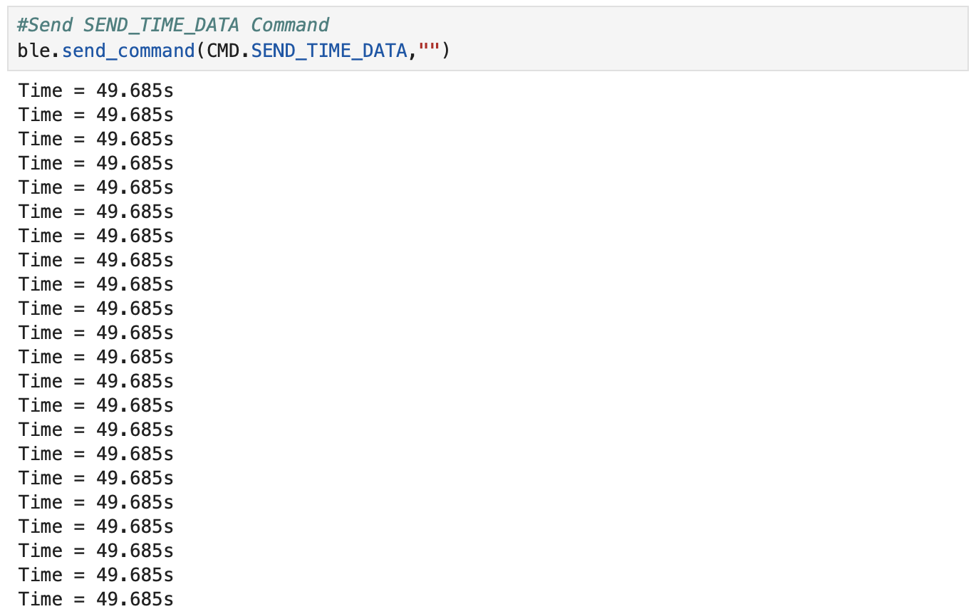
The following statements in Jupyter Notebook printed the timeSarray and the length of the array that was used to compute the data transfer rate.
The video below shows all of the times in the array.
Task 6: GET_TEMP_READINGS
A second array was added to store temperature readings from the Artemis board. The temperature array is the same size as the time array. The time and temperature readings were taken at the same time. The data is sent as an array to the computer using Jupyter Notebook.
The image below shows the Arduino IDE code.
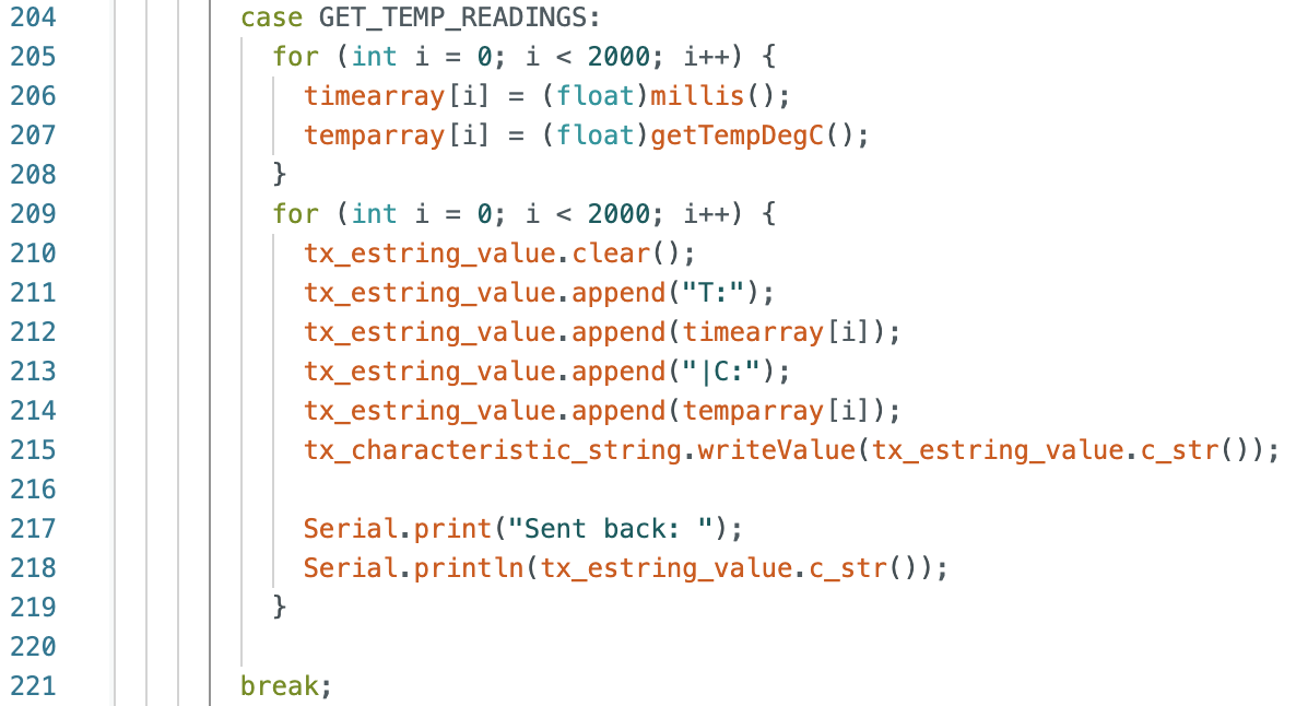
The image below shows the Jupyter Notebook command and some of the time and temperature outputs in the array.
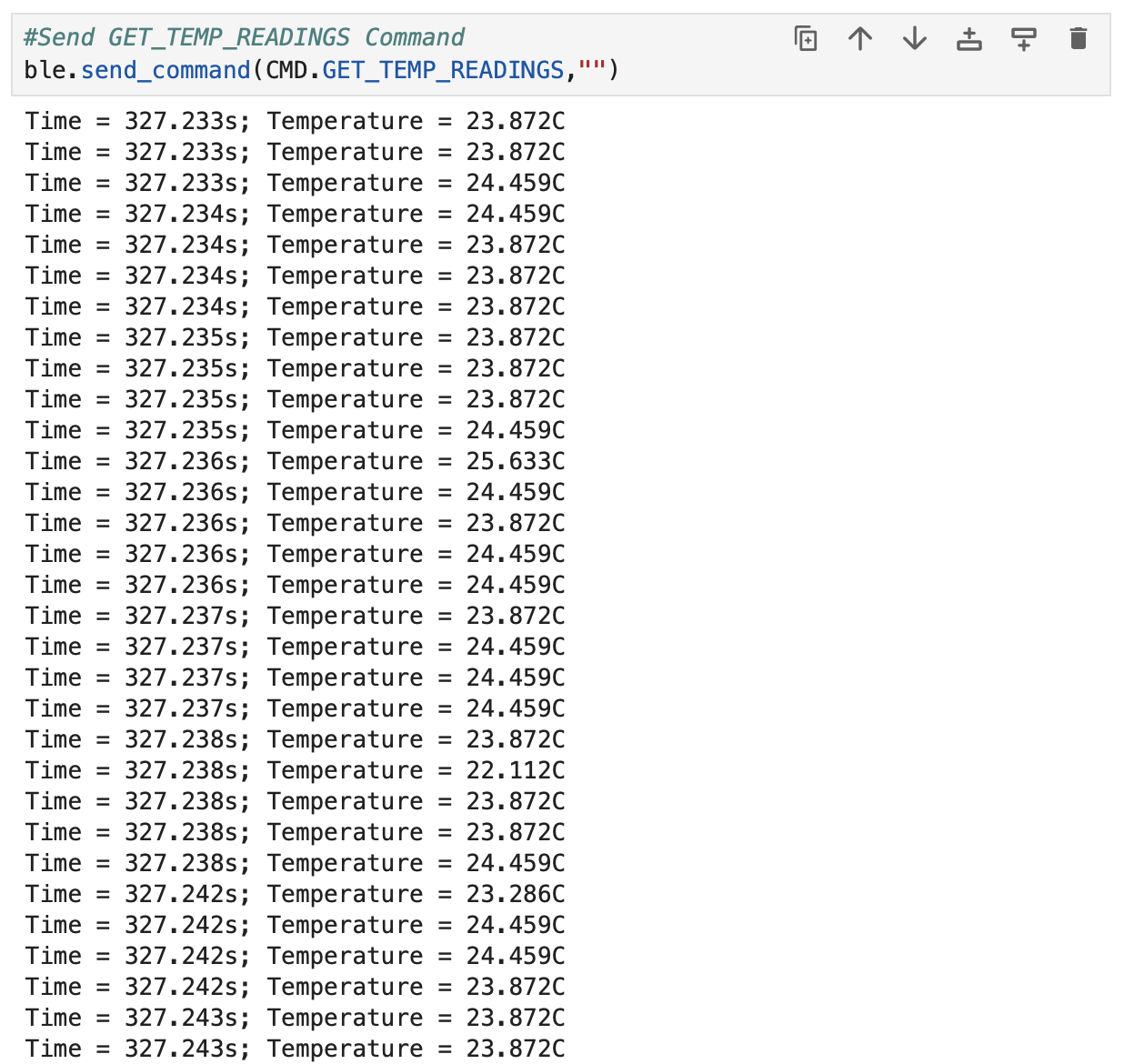
The video below shows all of the times and temperatures in the array.
Task 7: Discussion For Task 4 and Task 5
The method used in Task 4 involved sending the current time from the Artemis board to the computer. Each time was sent as an individual piece of data. The method used in Task 5 involved creating an array of times that was stored on the memory of the Artemis board and then sent to the computer to display the collected data.
The data transfer rate of the array method used in Task 5 (549600 bytes/second) is faster than the data transfer rate when sending individual pieces of data in Task 4 (1348.018 bytes/second).
An advantage of sending data individually as in Task 4 is that less memory on the Artemis board is being used, but the disadvantage is a slower data transfer rate. An advantage of sending data as an array as in Task 5 is that there is a faster data transfer rate, but a disadvantage is that more memory is being used on the Artemis to store the array.
The Artemis board has a maximum storage of 384 kB of RAM. If 16 bit values at 150 Hz were sampled every 5 seconds, 256 values would be stored before running out of memory on the Artemis board. The calculations can be found below.

5000 Level Task 1: Effective Data Rate And Overhead
I sent a message from the computer and received a reply from the Artemis board. The data rate for 5, 10, 20, 30, 40, 50, 60, 70, 80, 90, 100, 110, and 120 bytes was tested. The data rate for 5 bytes is 132.722 bytes/s and the data rate for 120 bytes is 2003.210 bytes/s. The plotted graph shows that as the number of bytes sent to the Artemis board increases, the data rate increases. Below are pictures of the Jupyter Notebook code, the graph, and the printed statements.
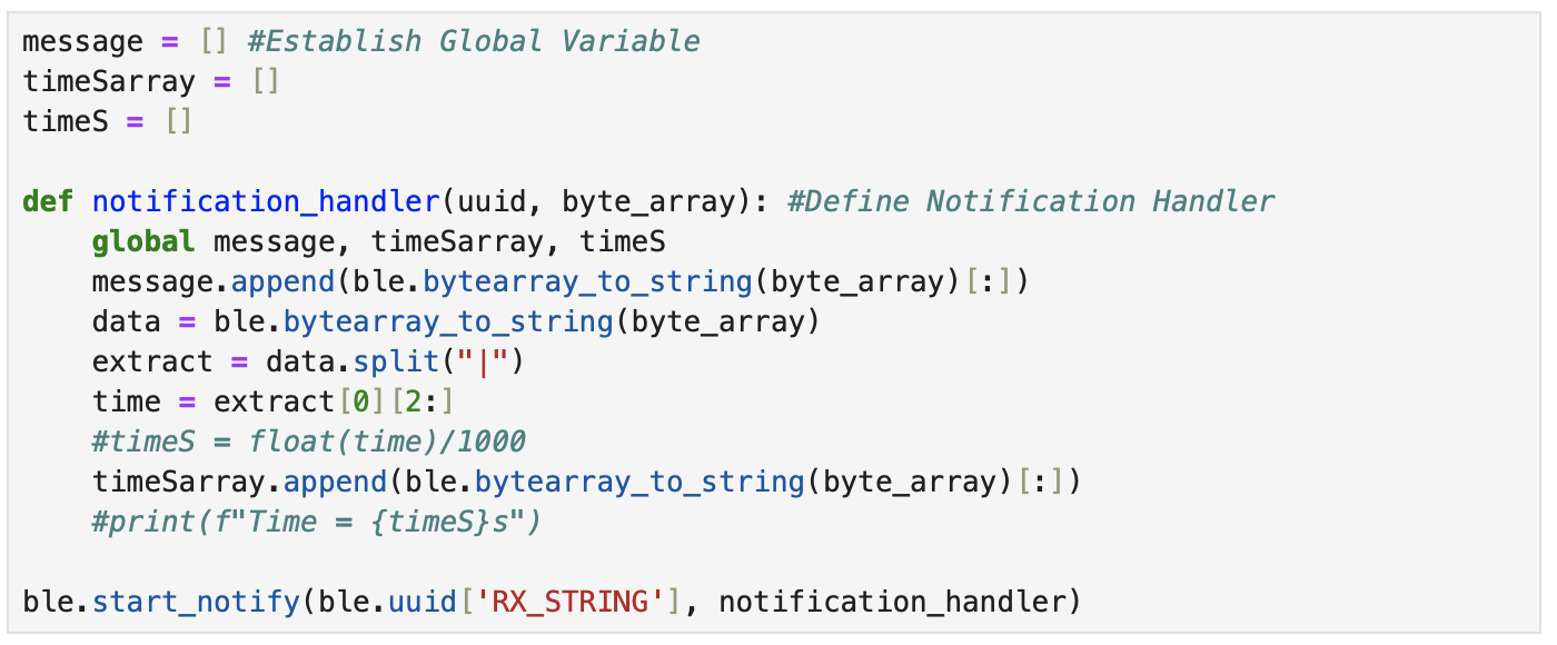


Additional graphs:


5000 Level Task 2: Reliability
I tested the reliability of sending data at a higher rate from the robot to the computer. To determine the reliability of the data I ran the GET_TEMP_READINGS command and compared the outputs printed in the Jupyter Notebook and the Arduino IDE Serial Monitor.
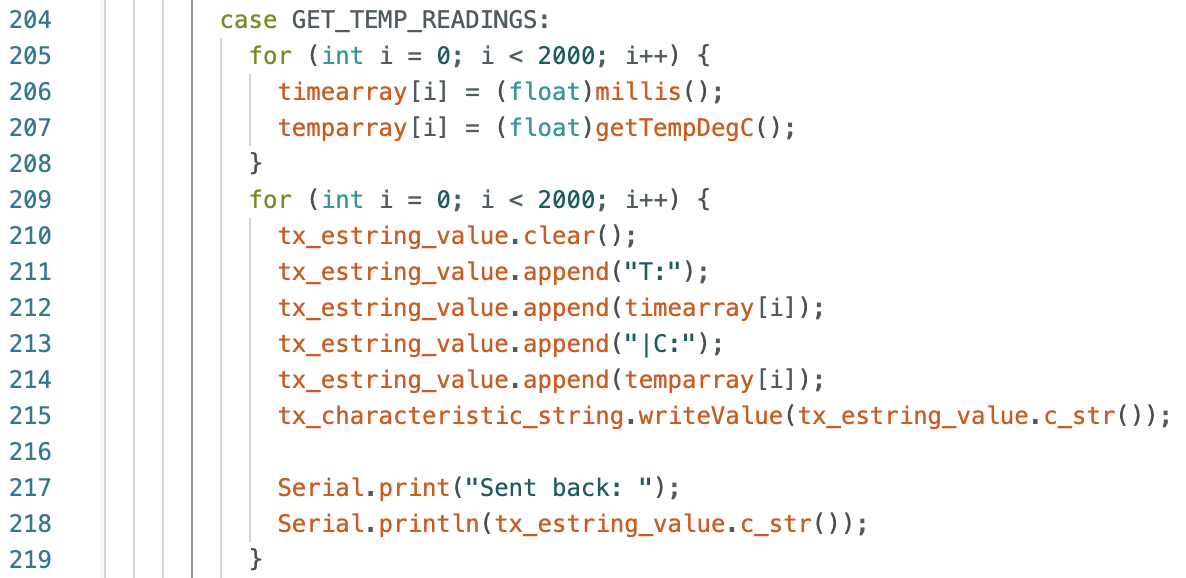
Outputs in the Jupyter Notebook (left) and the Arduino Serial Monitor (right):
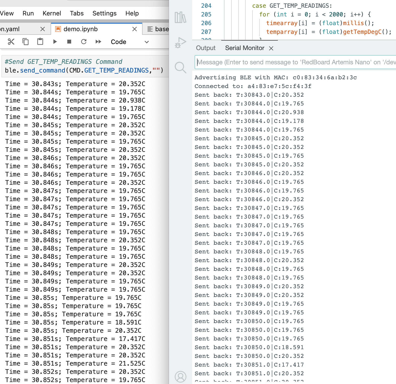
After looking at the outputs, the time and temperature readings on the computer are the same as the Artemis board and no data is missed. To confirm I copied and pasted the data from each window into Matlab variables titled time1 and temp1 for the Jupyter Notebook data, and time2 and temp2 for the Artemis data. I wrote a script to compare the corresponding time and temperature data and record how many data points are the same and how many are different. If there is a data point in the Jupyter Notebook that does not correspond to the Artemis board, or vice versa, an error message is displayed. The output variables in the workspace show that all data points are the same. The reliability is 100%.
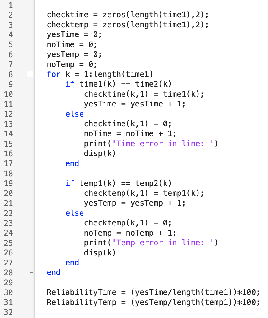
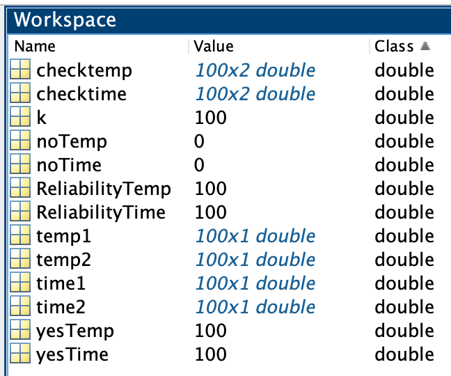
Discussion: Part 2
I learned how to use Bluetooth communication and UUIDs, between the Artemis board and computer. I did not experience any significant problems connecting to Bluetooth.
Lab 1 References
Thank you to all of the TAs that answered my questions. I referenced the past lab reports of Liam Kain, Rafael Gottlieb, Larry Lu, Julian Prieto, and Ignacio Romo.