Mikayla Lahr
I am a student in the Department of Mechanical and Aerospace Engineering at Cornell University. I am interested in robotics. This webpage contains all of the lab reports for MAE 5190 Fast Robots.
I am a student in the Department of Mechanical and Aerospace Engineering at Cornell University. I am interested in robotics. This webpage contains all of the lab reports for MAE 5190 Fast Robots.
The objective of the lab is to implement the Bayes Filter on the real robot. Due to noise when the robot is turning, only the update step of the filter will be be used during a 360 degree scan.
The lab materials include a fully assembled robot with SparkFun RedBoard Artemis Nano, Pololu TOF Distance Sensors, and a IMU Sensor.
Course lectures on sensor models, motion models, and the Bayes Filter were reviewed before starting the lab.
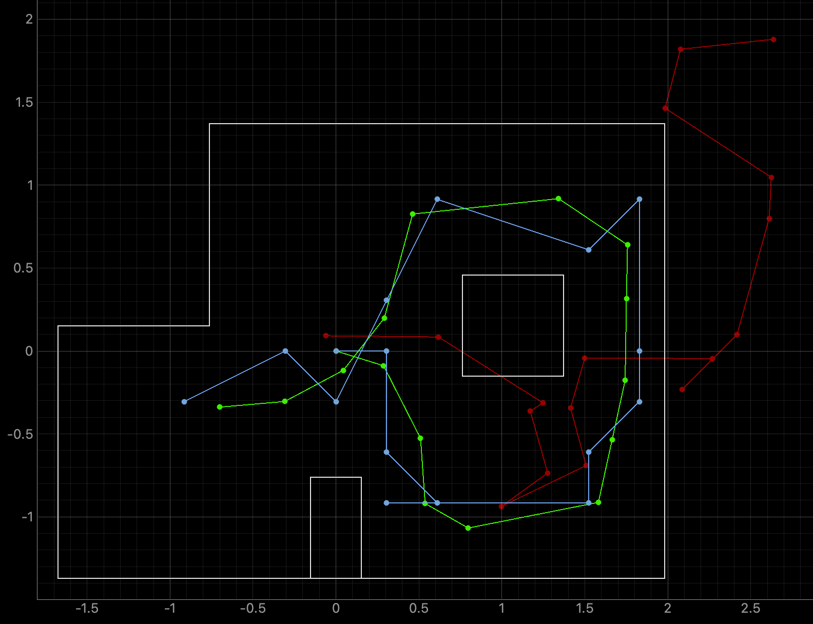
The first lab task was to run the provided Bayes Filter simulation. The lab11_sim.ipynb file was downloaded and a screenshot of the final result is below as well as a link to the data from the simulation. The red line is odometry, the green line is the ground truth, and the blue line is the belief. The map is a three dimensional grid (x, y, theta). The dimension of x is 12, the dimension of y is 9, and the dimension of theta is 18.
To perform localization on the robot the Arduino IDE code from Lab 9: Mapping was used to rotate the robot 360 degrees. The setAngle was changed from 10 degrees, used in Lab 9, to 20 degrees for Lab 11. I removed some of the append statements in case SEND_ORIENTATION_DATA to only send time, angle in 20 degree increments, and the distance readings at each angle increment. In the main while loop I changed how I stored the distance data and yaw readings. I initially stored the readings as variables before assigning them to an array at each 20 degree increment. The code is below.
ORIENTATION_CASE:
SEND_ORIENTATION_DATA:
While Loop:
The RIGHT_MOTOR() and LEFT_MOTOR() functions used did not change from Lab 9.
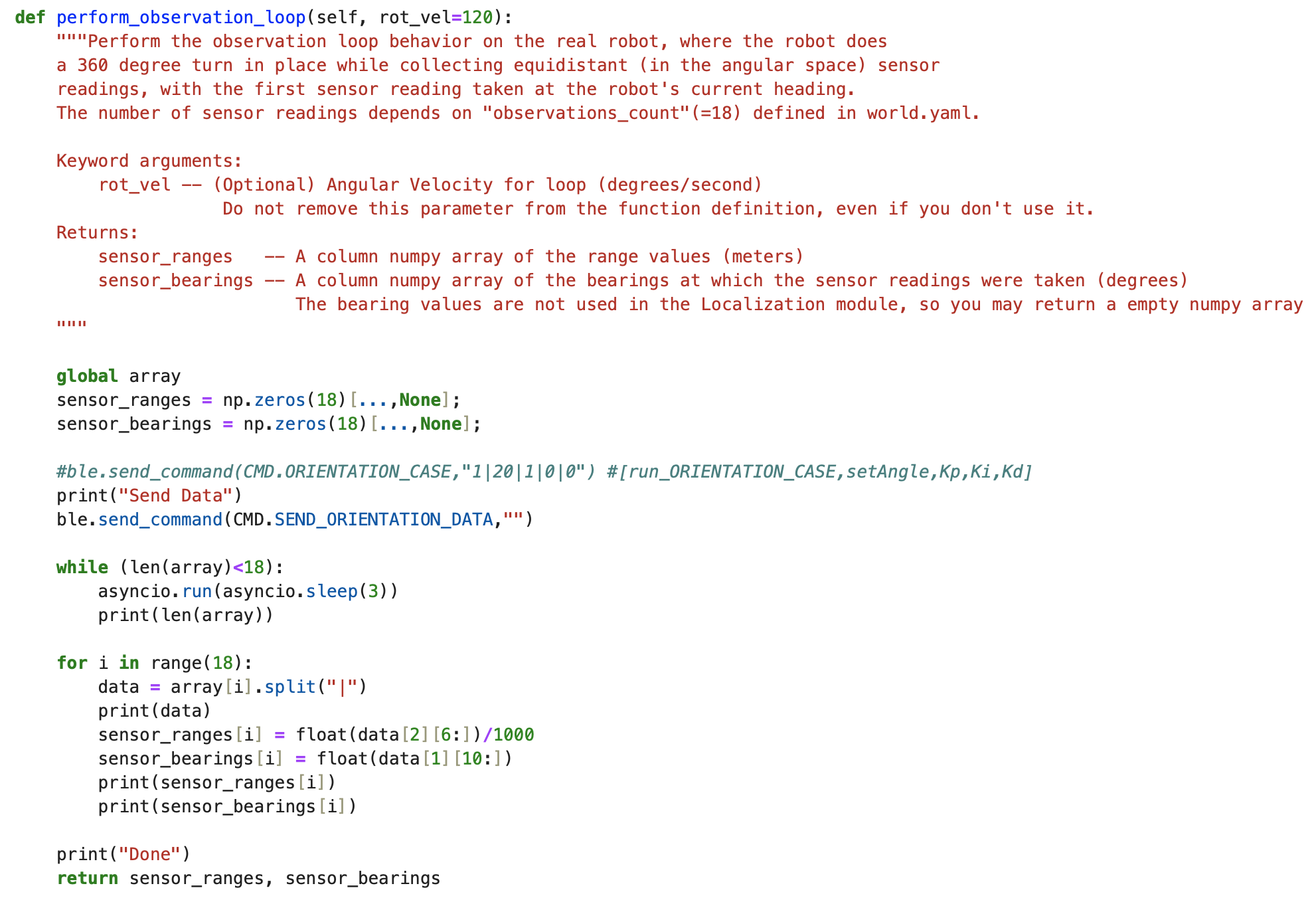
The code lab11_real.ipynb was downloaded and opened in Jupyter Notebook. The function perform_observation_loop was written to sort through the collected data from one rotation. First arrays are established and then the command to send orientation data is run. The asynicio function was used to run the while loop until 18 data readings are sent over Bluetooth. The for loop assigns the angle readings to the sensor_bearings array and the distance readings, converted from millimeters to meters, to the sensor_ranges array. Initially, I put the command to run the ORIENTATION_CASE inside of the perform_observation_loop function, but I decided to run the rotation first before calling the function. Removing the command to run ORIENTATION_CASE from inside of the function allowed me to more easily turn on/off the rotation.
The function perform_observation_loop is below:
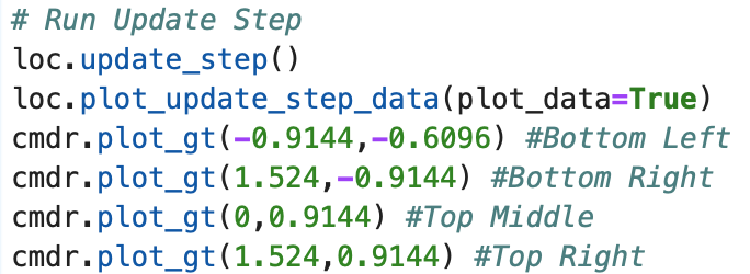
The command to run ORIENTAION_CASE is below:

The results of rotating the robot at the four marked positions are below. The four marked positions include: (-3ft, -2ft, 0deg), (0ft, 3ft, 0deg), (5ft, -3ft, 0deg), and (5ft, 3ft, 0deg). The robot was run around 4-5 times at each point. Two runs for each point are shown below. The ground truth is plotted as the green dot and is the location where the robot rotated. The belief of the robots position is plotted as the blue dot. The ToF sensor used to collect distance readings was located on the front of the robot, between the left and right sides of the robot. When the robot was at zero degrees the ToF sensor was pointed towards the rightside wall. The robot turned counterclockwise in the same manner as in Lab 9. The Jupyter Notebook code to plot each Ground Truth value is below:
Graphs for the Belief (blue) and the Ground Truth (green):
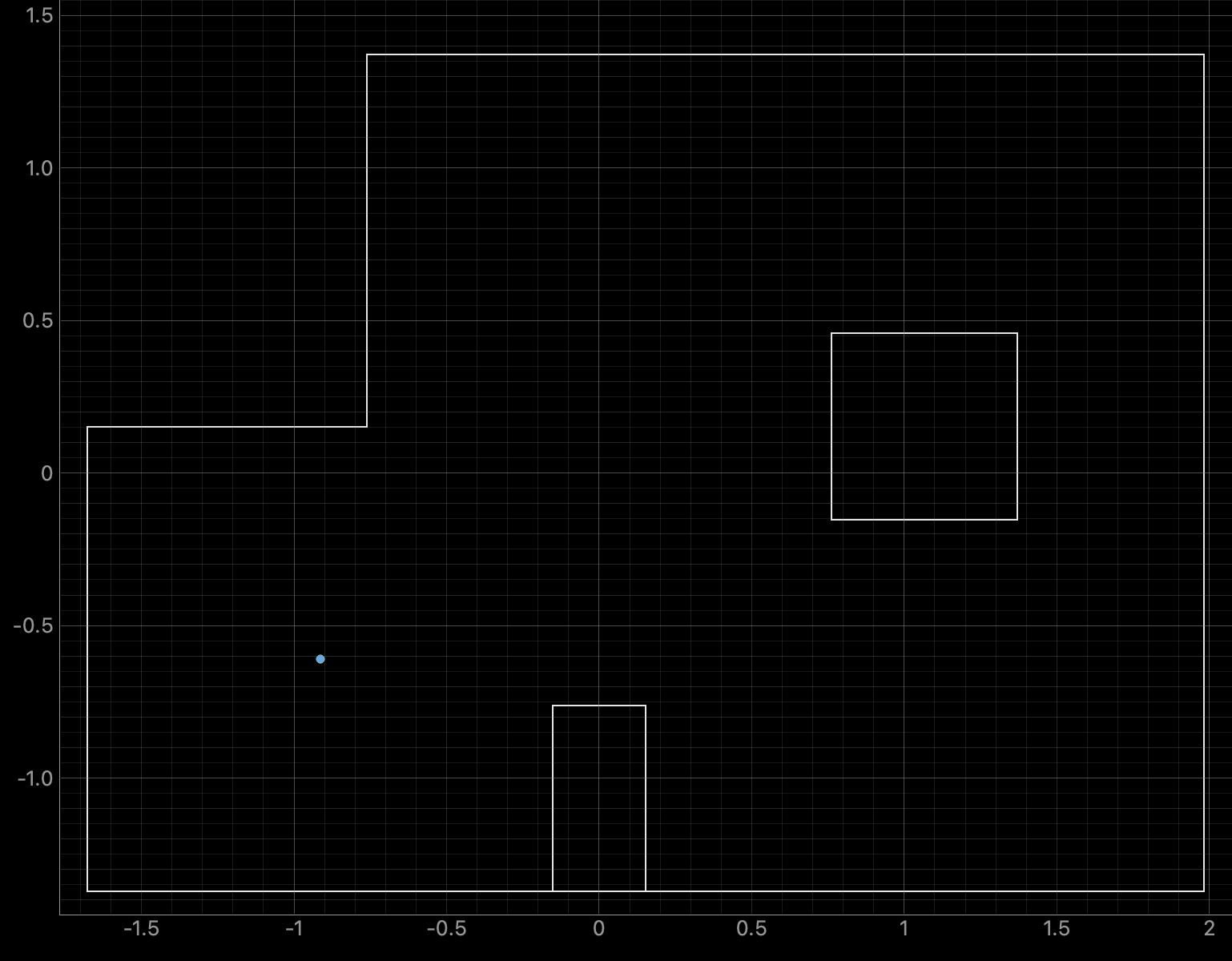
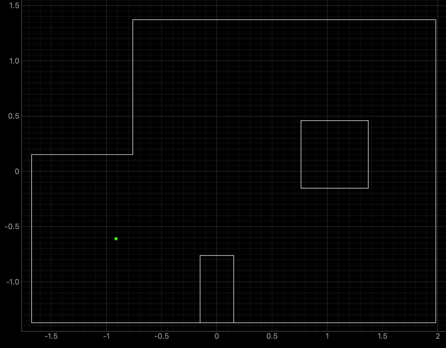
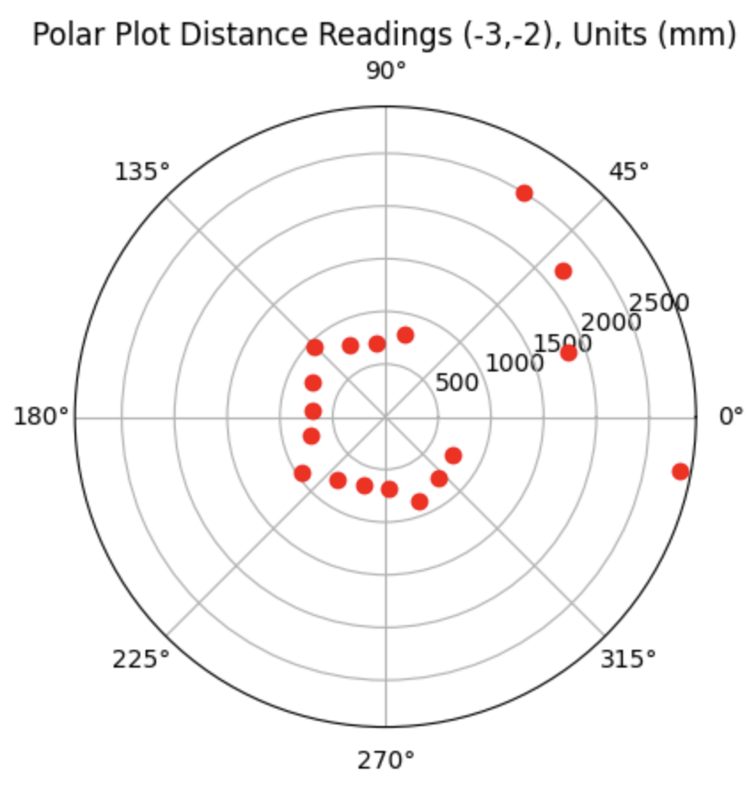
For run 1 of the bottom left point, the Belief was at the same point as the Ground Truth. As can be seen in the below polar plot, the robot sensed the surrounding walls very well. I reran the rotation several (5) times and this point had the most rotations result in the Belief being the same as the Ground Truth. This is a result of the several walls surrounding the robot when rotating. The next run shows one of the runs where the Belief was different then the Ground Truth.
Belief Data:

Polar Plot and recorded data below:
Graph for the Belief (blue) and the Ground Truth (green):
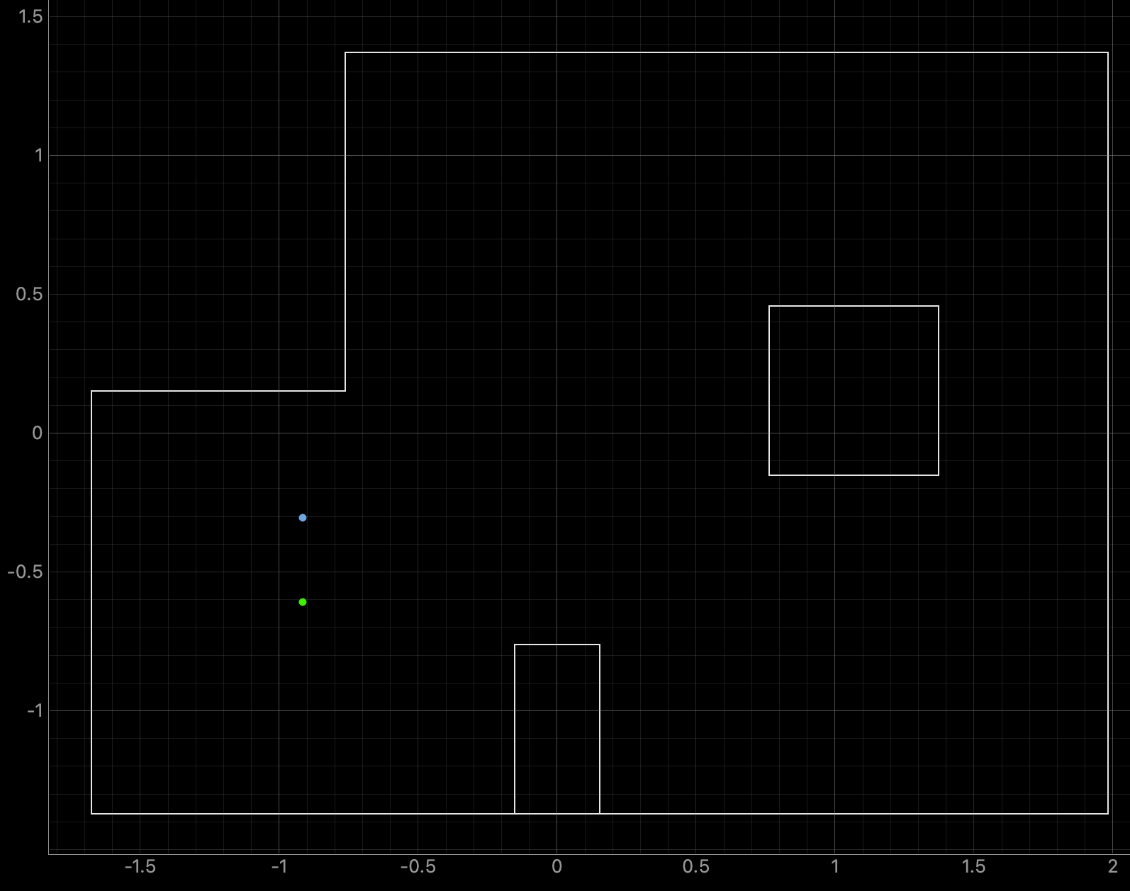
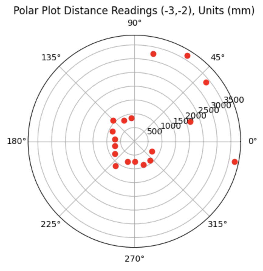
For run 2 of the bottom left point, the Belief was 0.3050 meters above the Ground Truth. As can be seen in the below polar plot, the walls were not as defined as in the previous run, resulting in the error in localization.
Belief Data:

Polar Plot and recorded data below:
Graphs for the Belief (blue) and the Ground Truth (green):
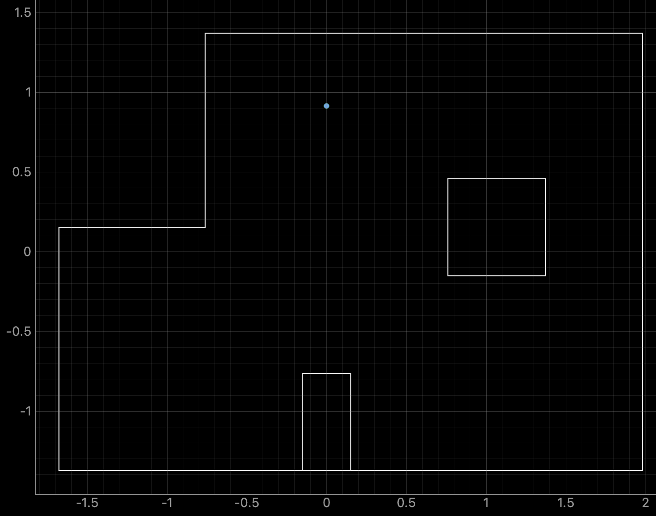
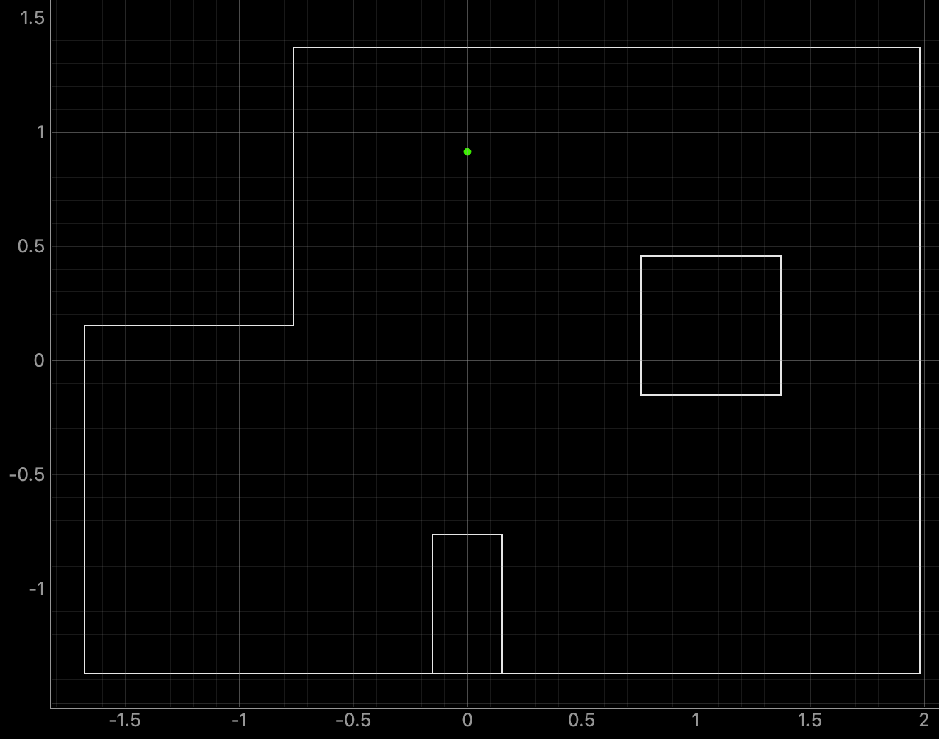
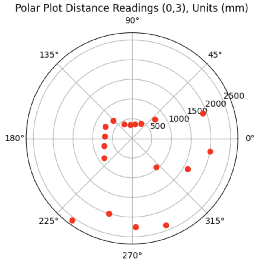
For run 1 of the top middle point, the Belief was at the same point as the Ground Truth. I was surprised to achieve this result as there are not a lot of nearby walls to use for localization and I suspected that this would be the hardest point to localize. As can be seen in the below polar plot, the robot was able to sense the surrounding walls and obstacles.
Belief Data:

Polar Plot and recorded data below:
Graph for the Belief (blue) and the Ground Truth (green):
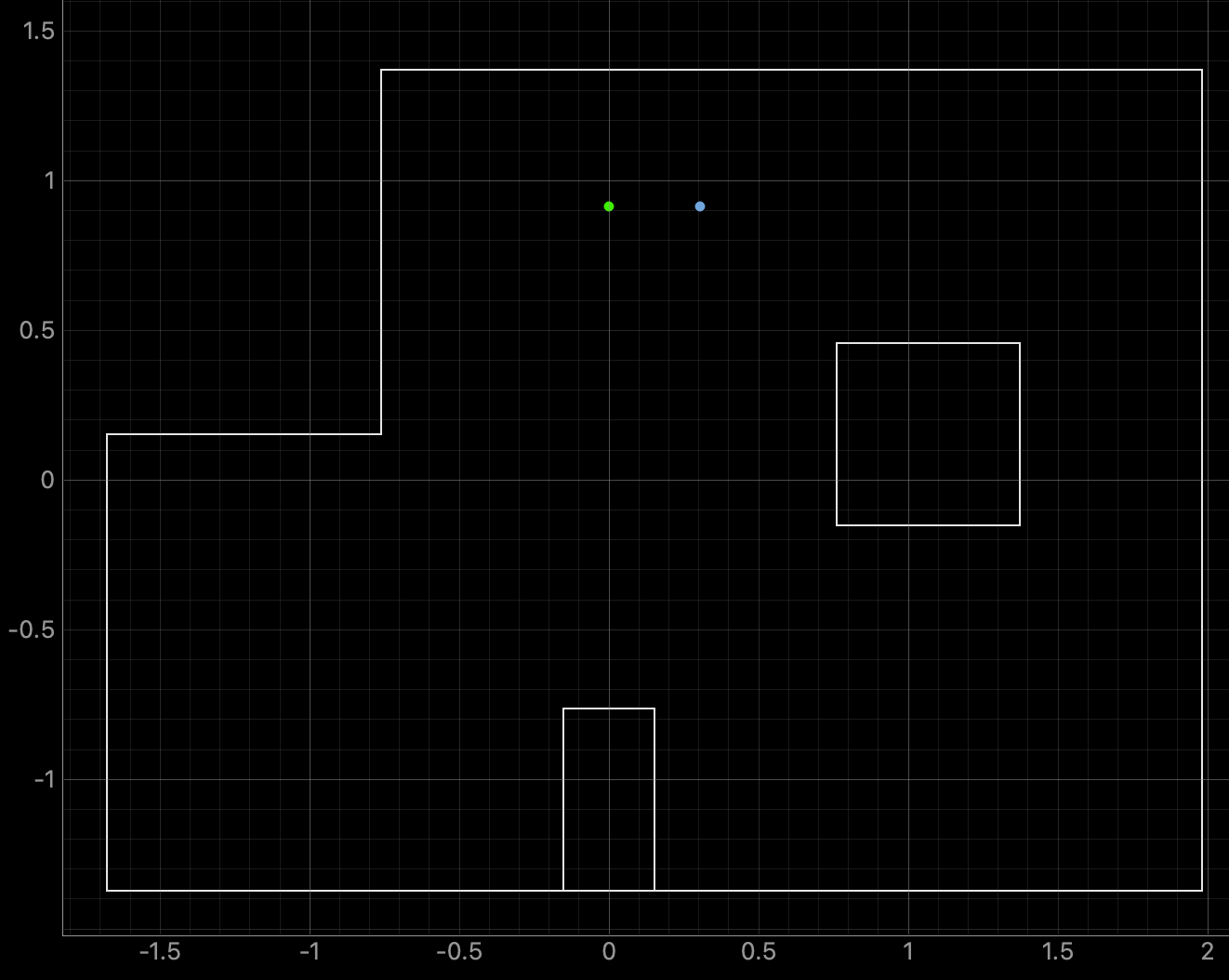
For run 2 of the top middle point, the Belief was 0.3050 meters to the right of the Ground Truth. The robot did not turn as well as in the previous run and the left side wall was not as accurately sensed. The results are shown in the below polar plot. Despite the non-ideal rotation of the robot, the location of the robot was still fairly close to the Ground Truth value.
Belief Data:

Polar Plot and recorded data below:
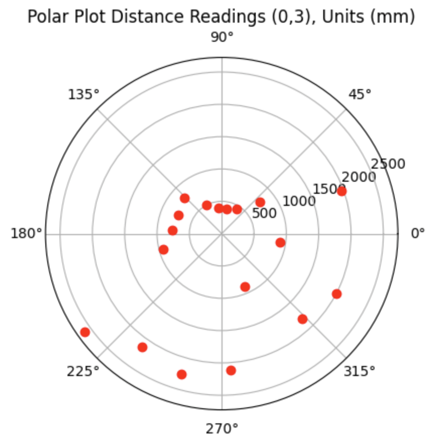
Graphs for the Belief (blue) and the Ground Truth (green):
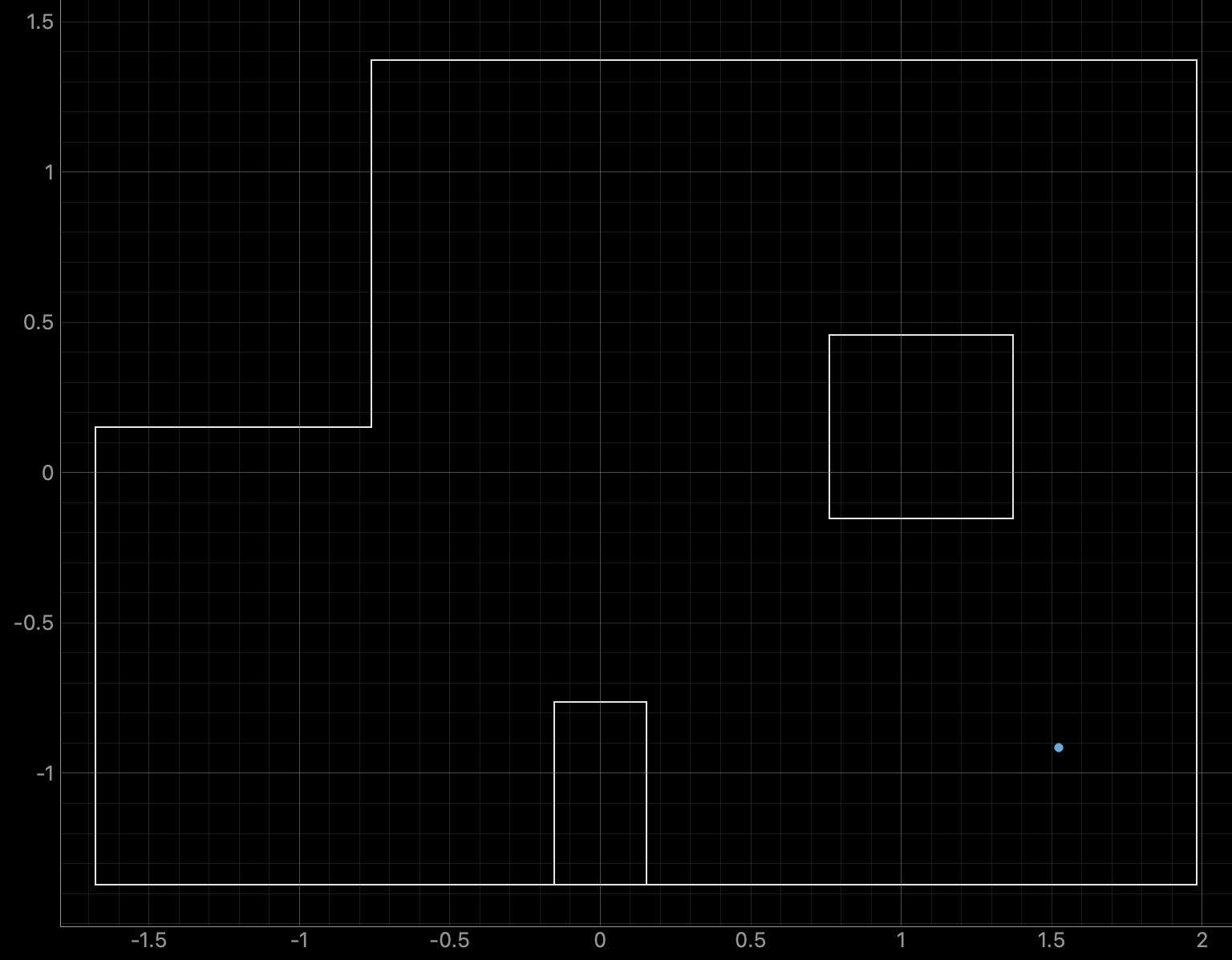
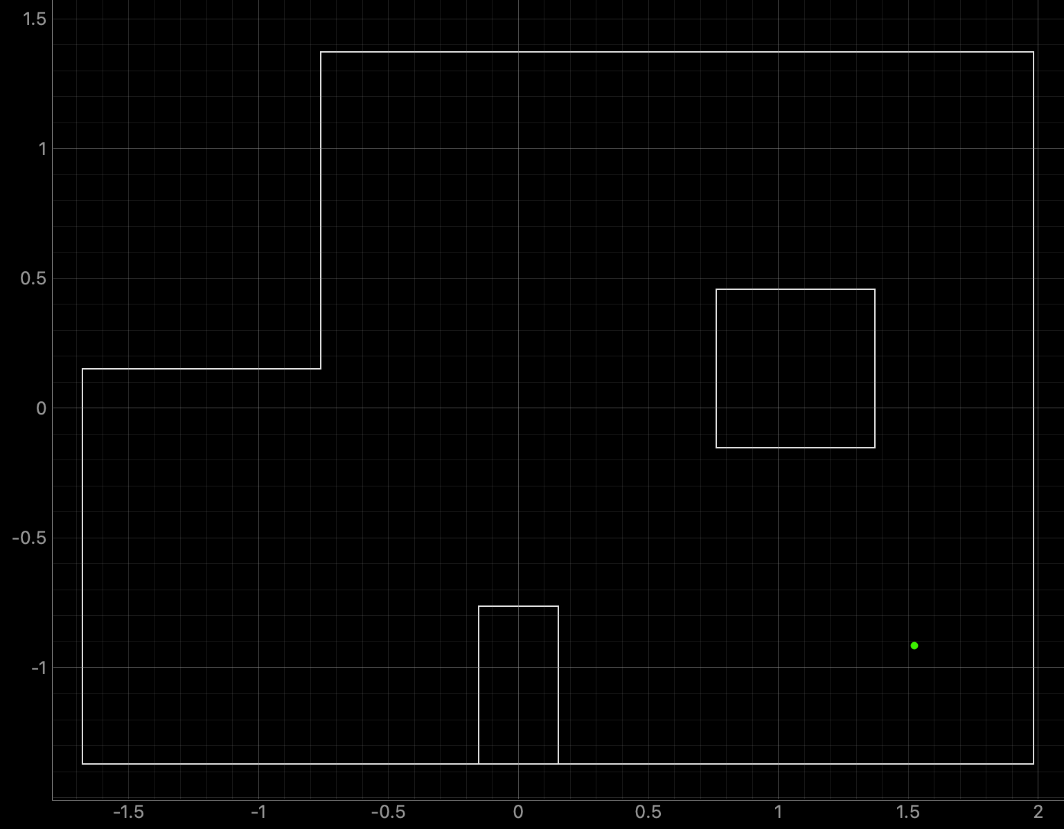
For run 1 of the bottom right point, the Belief was at the same point as the Ground Truth. As can be seen in the below polar plot, the robot rotated well and was able to sense the surrounding walls and obstacles.
Belief Data:

Polar Plot and recorded data below:
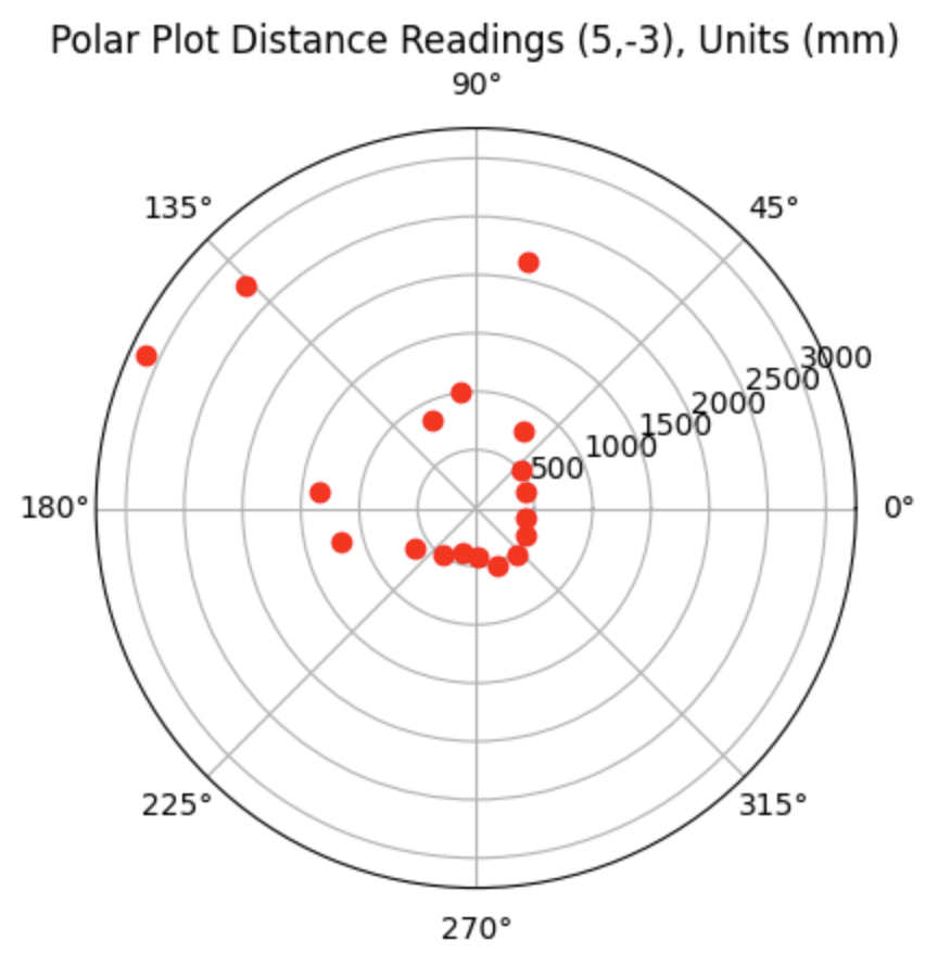
Graph for the Belief (blue) and the Ground Truth (green):
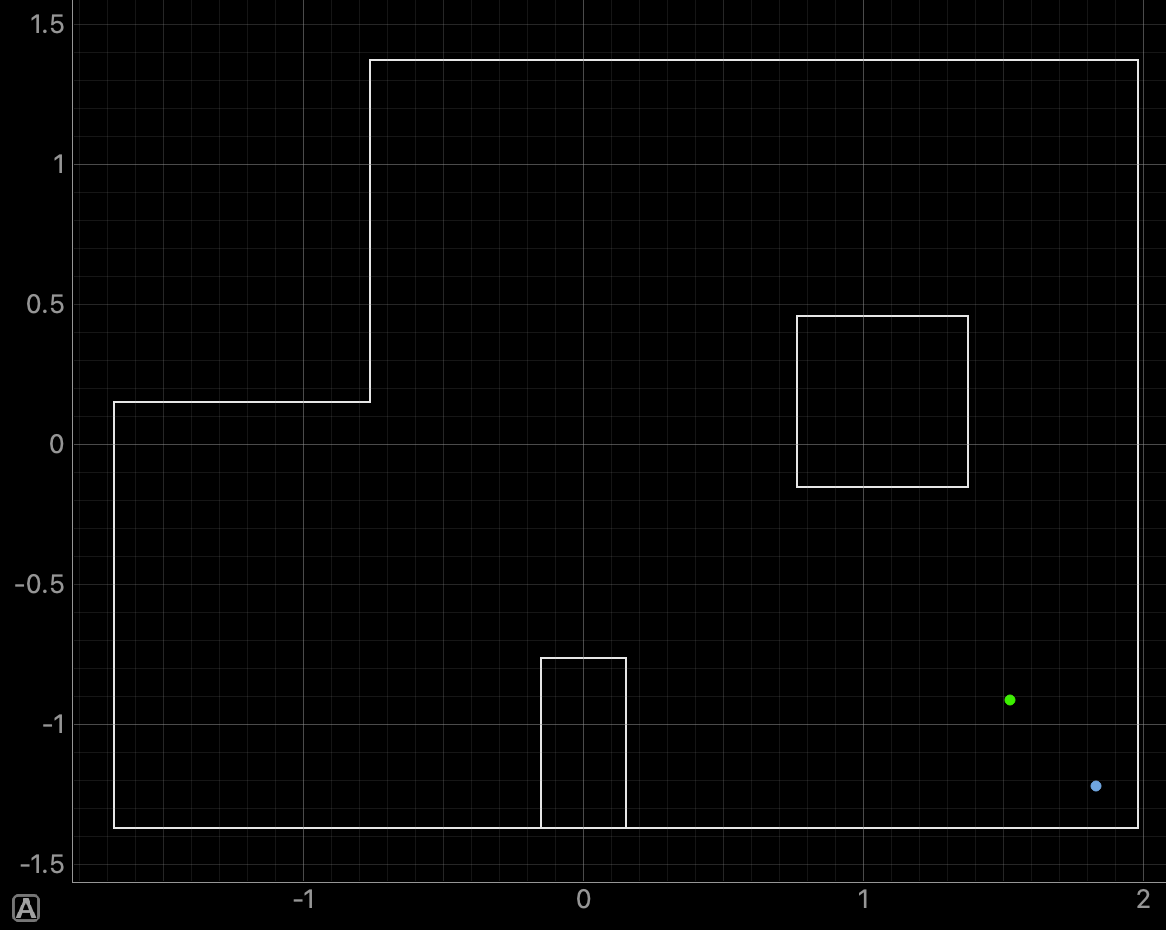
For run 2 of the bottom right point, the Belief was located 0.3050 meters to the right and 0.3046 meters below the Ground Truth. As can be seen in the below polar plot, for this run the plotted edges of the walls are not as straight as in the previous run.
Some runs of the robot for the bottom right point resulted in a Belief that was plotted around (-0.8m, 0.2m) as the corner outside of the map resembled the lower right corner inside of the map. I found it surprising that the Belief would be plotted outside of the map and discussed the results with a TA. To address this issue the probability that the robot is located outside of the map can be set to zero in the Bayes Filter.
Belief Data:

Polar Plot and recorded data below:
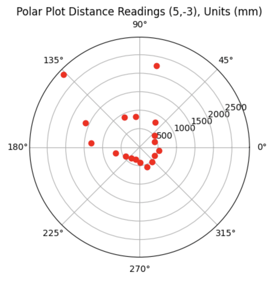
Graph for the Belief (blue) and the Ground Truth (green):
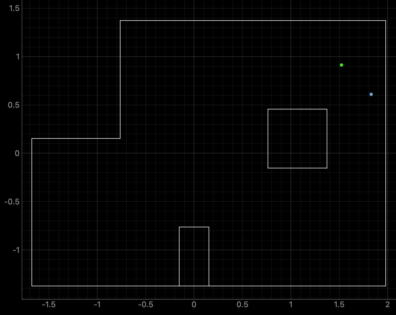
For run 1 of the top right point, the Belief was located 0.3050 meters to the right and 0.3044 meters below the Ground Truth. As can be seen in the below polar plot the robot had difficulty achieving the correct distance measurements for the right side wall, which may have impacted the localization Belief.
Belief Data:

Polar Plot and recorded data below:
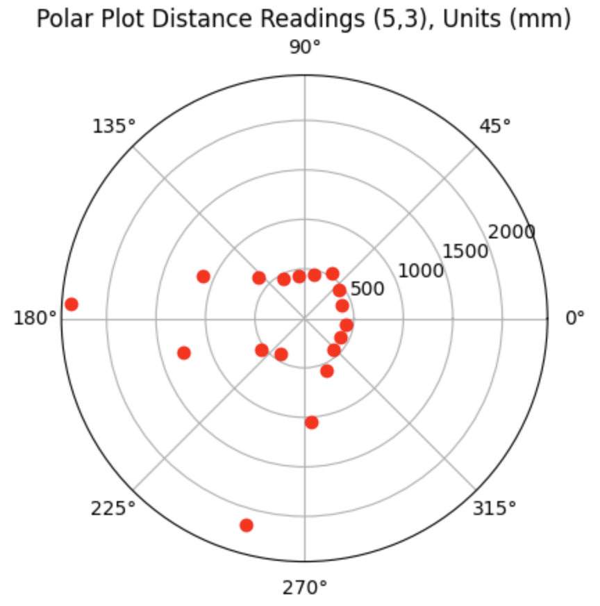
Graph for the Belief (blue) and the Ground Truth (green):
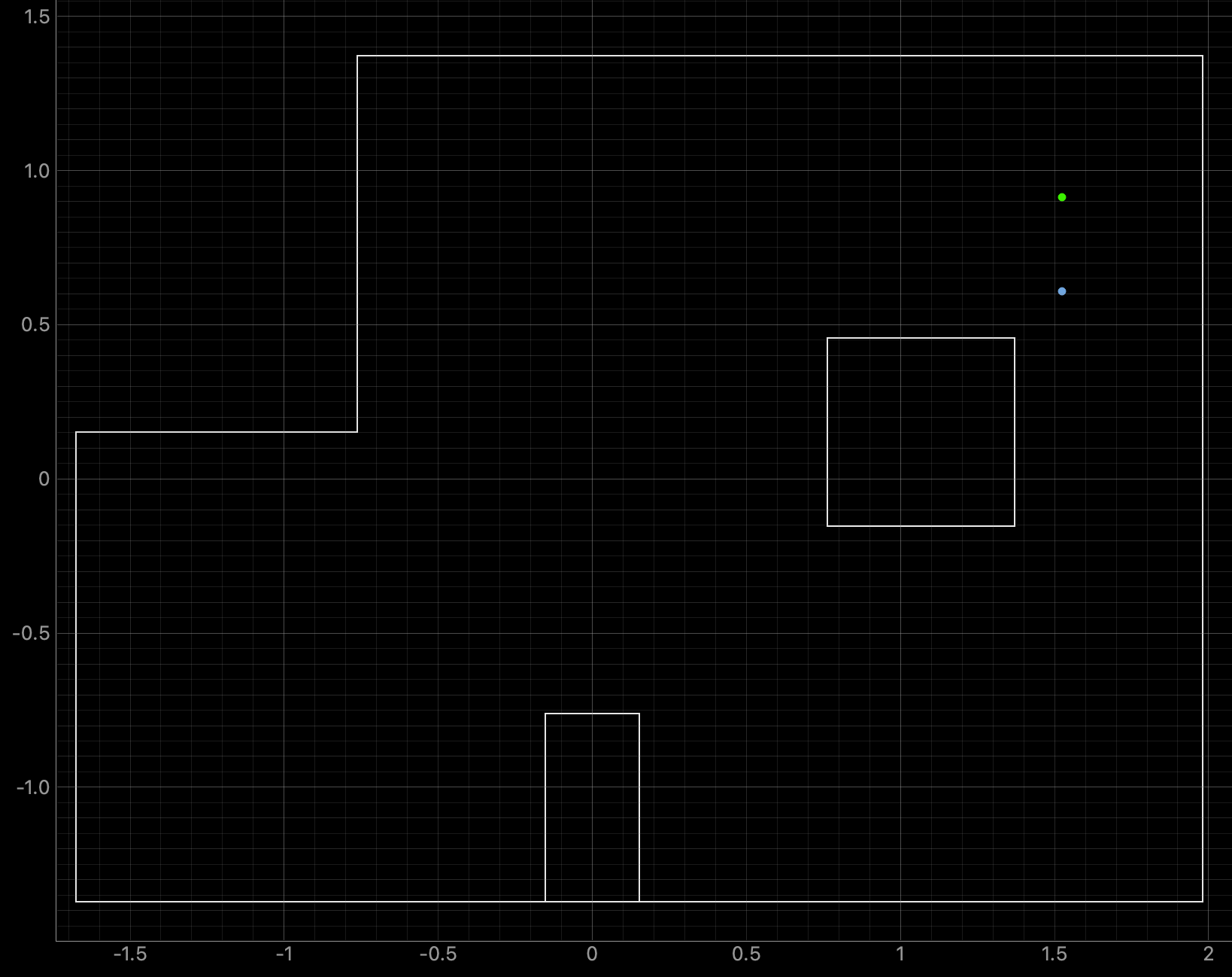
For run 2 of the top right point, the Belief was located 0.3044 meters below the Ground Truth. As can be seen in the below polar plot the robot again had difficulty achieving the correct distance measurements for the right side wall, which may have impacted the localization Belief.
Belief Data:

Polar Plot and recorded data below:
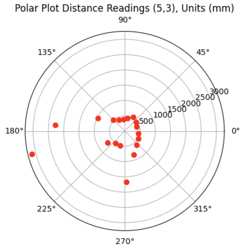
Overall, the localization implemented on the robot was able to achieve Belief results that aligned with the Ground Truth values for 3 out of the 4 tested points (bottom left, top middle, bottom right). I also included non-ideal runs in the lab report to show that even for non-ideal rotations the robot would still localize fairly well. The bottom left point had the most number of rotations (4/5) that resulted in the Belief being in the same location as the Ground Truth. This is compared to the Top Middle having 1/4, Top Right having 0/4, and the Bottom Right having 2/4. I suspect that the Top Right did not achieve any Belief values that were the same as the Ground Truth values because the rotations at that point did not adequately pick up on the straight edges of the wall.
Thank you to all of the TAs that answered my questions. I referenced the past lab reports of Liam Kain, Rafael Gottlieb, Larry Lu, Julian Prieto, and Ignacio Romo.
The objective of the lab is to use the Bayes Filter to implement grid localization.
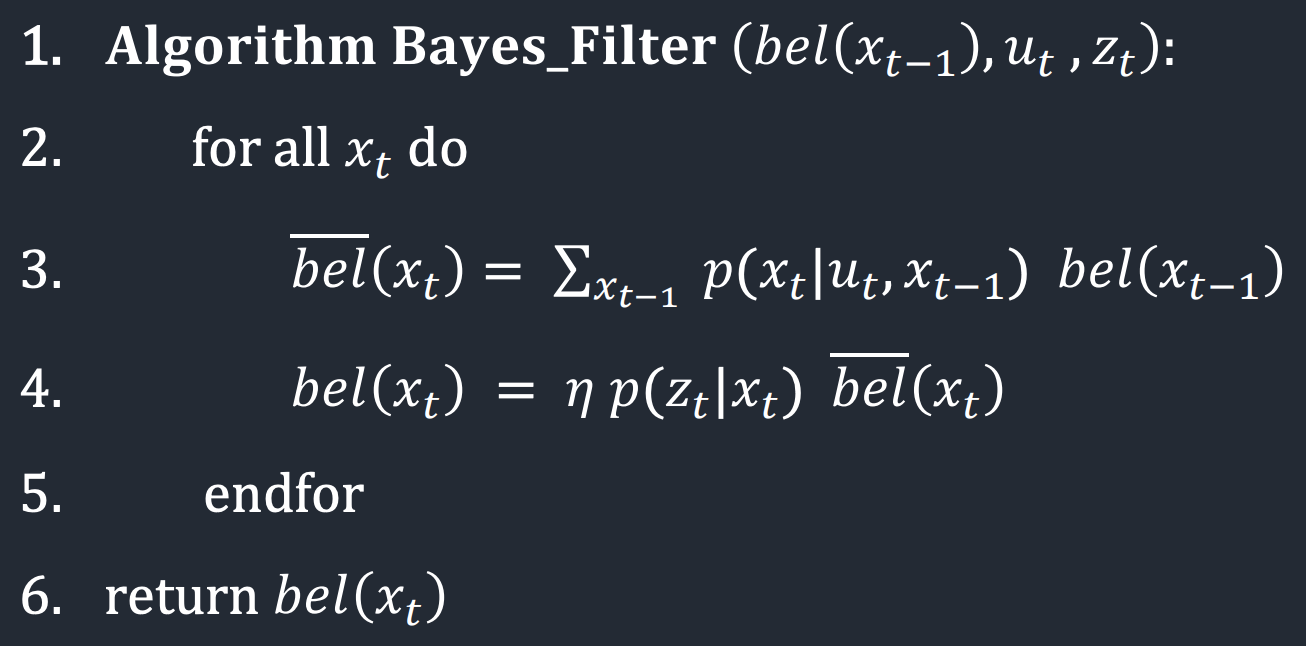
Before starting the lab, I familiarized myself with how the Bayes Filter worked and how to implement the Bayes filter for the robot in simulation. Localization and of the robot determines where the robot is in the enviroment. There is a predition and update step of the Bayes filter. The prediction step uses the control input and accounts for the noise from the actuator to predict the new location of the robot. After the prediction step, the robot rotates 360 degrees gathering distance measurement data. The update step uses the gathered distance measurements to determine the real location of the robot. The Bayes Filter from Lecture 16 is below:
The dimensions of each grid cell in the x, y, and theta axes are 0.3048 meters, 0.3048 meters, and 20 degrees. The grid is (12,9,18) in three dimensions, totalling 1944 cells. The discritized grid map is:
Five functions were written to run the Bayes Filter as outlined below.
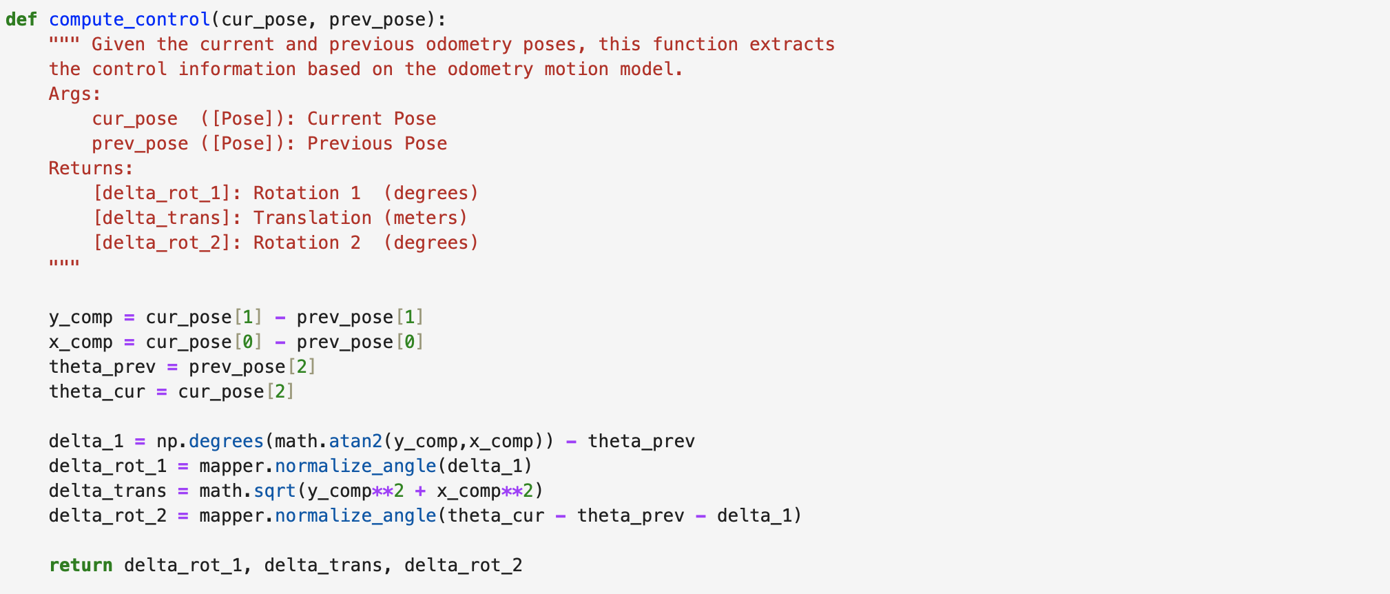
The control information from the robot is used to find the first rotation, translation, and second rotation. The inputs include the current position (cur_pose) and the previous position (prev_pose). The return values include the first rotation (delta_rot_1), the translation (delta_trans), and the second rotation (delta_rot_2). The Lecture 17 slide with the equations to find the odometry model parameters is below:
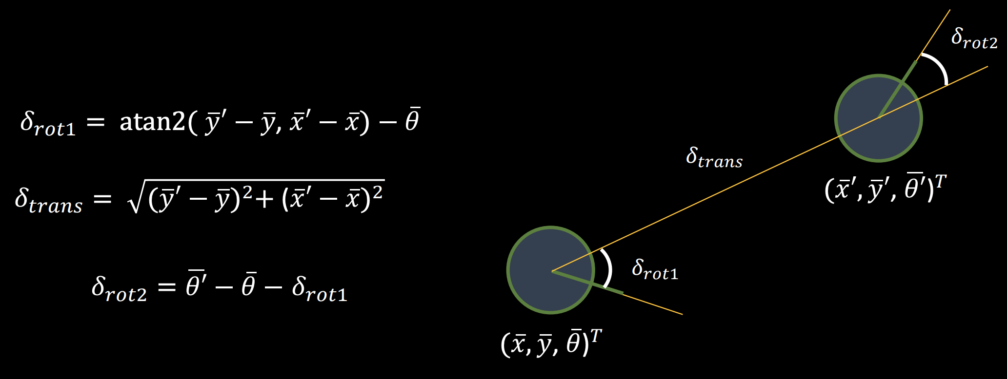
The above equations were modeled in Jupyter Notebook. The code is found below. First the differences in the y and x positions are found (y_comp and x_comp). Then the normalized rotations are calculated as well as the translation.
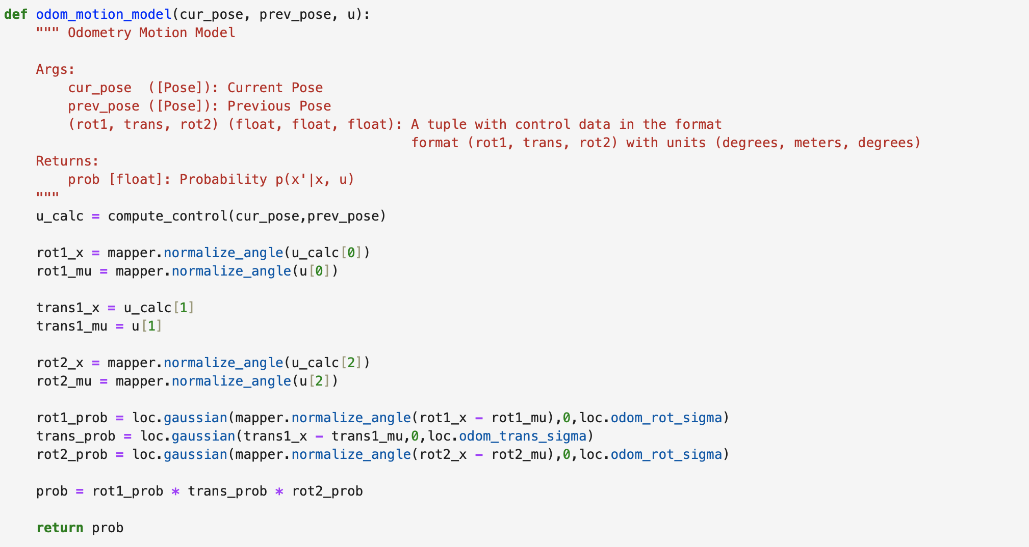
The odometry motion model finds the probability that the robot performed the motion that was calculated in the previous step. The inputs include the current position (cur_pose), previous position (prev_pose), and odometry control values (u) for rotation 1, translation, and rotation 2. The return value is the probablility ( p(x'|x,u) ) that the robot achieved the current position (x'), knowing the previous position (x) and odometry control values (u). A Gaussian distribution is used. Each motion is assumed to be an independent event. The probability of each event is then multiplied together to find the probability of the entire motion. The Jupyter Notebook code is found below.
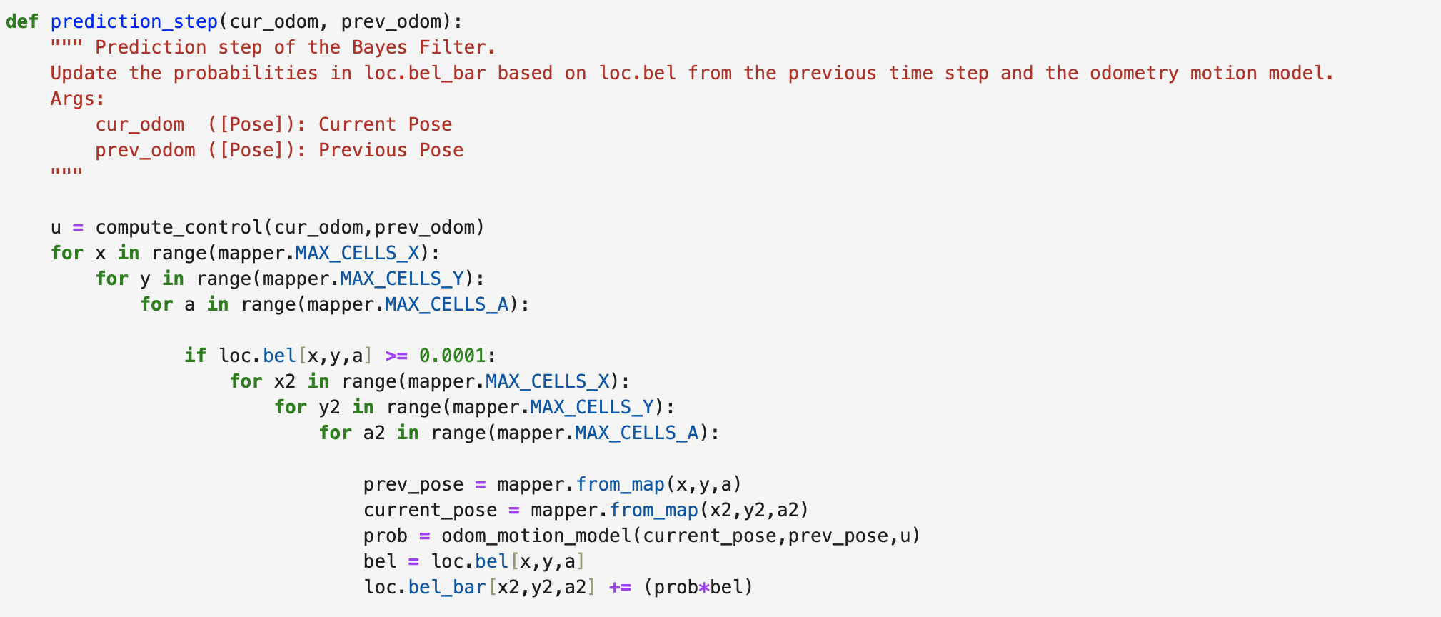
The prediction step of the Bayes Filter as implemented in Jupyter Notebook uses six for loops to calculate the probability that the robot moved to the next grid cell. The inputs include the current odometry position (cur_odom) and the previous odometry position (prev_odom). The if statement in the pediction step code is used to speed up the filter. If the belief is less than 0.0001 than the three remaining for loops will not be entered as the robot is unlikely to be in the remaining grid cells. If the belief is greater than or equal to 0.0001 the probability will be calculated. The code for calculating the probability is below.
The sensor model function finds the probability of the sensor measurements, modelled as a Gaussian distribution. The length of the array is 18 as the robot measures 18 different distance reading values. The input includes the 1D observation array (obs) for the robot position. The function returns a 1D array of the same length including the likelihood of each event (prob_array). The Jupyter Notebook code is below.

The update step calculates the belief of the robot for each grid cell. The probability ( p(z|x) ) is multiplied by the predicted belief (loc.bel_bar) to find the belief (loc.bel). The belief is then normalized. The code can be found below.

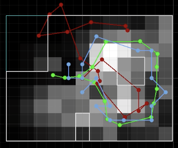
Two runs of the Bayes Filter simulation are found below. The green line is the ground truth, the blue line is the belief, and the red line is the odometry measurements. The lighter grid cells represent a higher belief. For both runs the ground truth and the belief are close together. Both runs were 15 iterations.
Run 1 Final Graph:
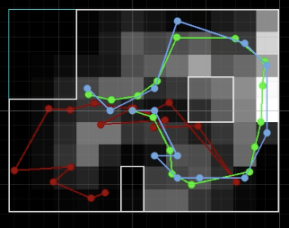
Run 2 Final Graph:
Thank you to all of the TAs that answered my questions. I referenced the past lab reports of Liam Kain, Rafael Gottlieb, Larry Lu, Julian Prieto, and Ignacio Romo.
The objective of the lab is to use yaw angle measurements from the IMU sensor and distance readings from the ToF sensor to map a room. The map will be used during localization and navigation tasks. Map quality depends on how many readings are obtained and the separation between each reading during each rotation.
The lab materials include a fully assembled robot with SparkFun RedBoard Artemis Nano, Pololu TOF Distance Sensors, and a IMU Sensor.
Course Lecture 2 on transformation matrices was reviewed before starting the lab.
Option 2: Orientation Control was chosen as the PID controller for the lab. The PID controller results in the robot performing on-axis turns in 10 degree increments. The ToF sensor used to collect distance readings is located on the front of the robot between the left and right motor sides.
The Arduino code for the created ORIENTATION_CASE in the while loop is found below.
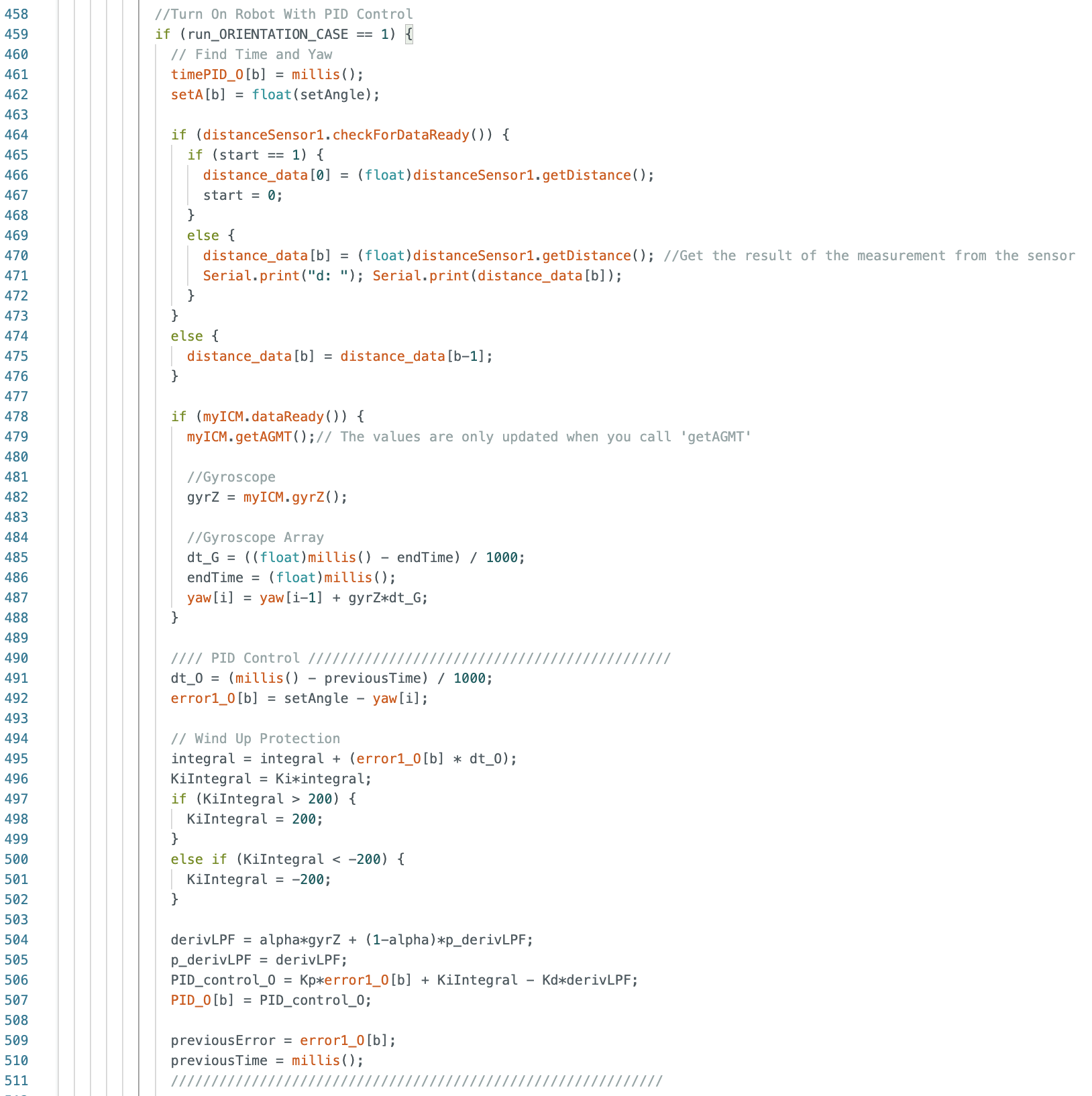
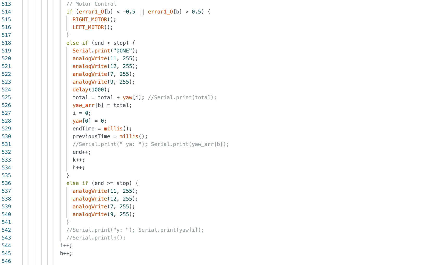
First the distance is found using the readings from the ToF sensors, then the yaw angle is found using the IMU sensor. The PID controller value is used in the RIGHT_MOTOR and LEFT_MOTOR functions to determine the motor input value. If the error between the current yaw angle and the setAngle (10 degrees) is less than -0.5 degrees or greater than 0.5 degrees then the RIGHT_MOTOR and LEFT_MOTOR functions will run. The "stop" variable is set to be 360 divided by the "setAngle" variable, which is equal to 10. The results in stop = 36 increments. If variable "end" is less than "stop" the robot will stop for one second. I stopped the robot for one second to ensure that the ToF sensor is pointed towards a fixed point in space. The total yaw angle is recorded by adding the current total to the current yaw value (yaw_arr). The yaw value is then set to zero for the next iteration of the while loop. Resetting the yaw value for the IMU sensor reduces gyroscope drift. If the "end" value is greater than or equal to the "stop" value the robot will stop and no new data will be recorded into the yaw_arr array.
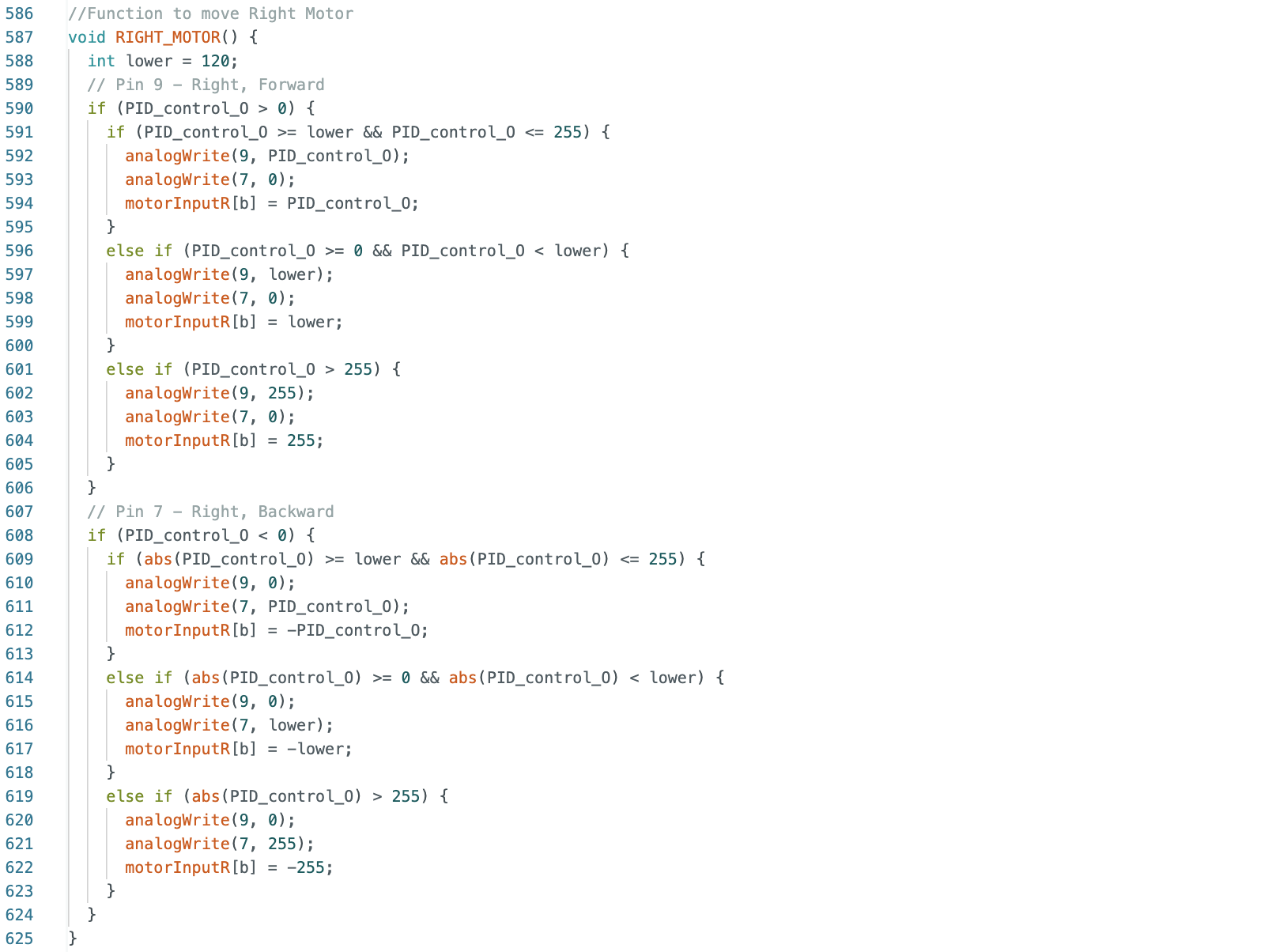
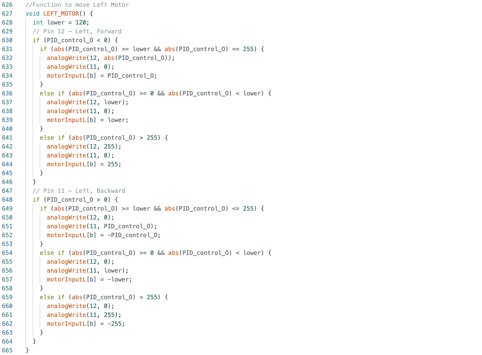
The RIGHT_MOTOR and LEFT_MOTOR functions called from the code above are found below.
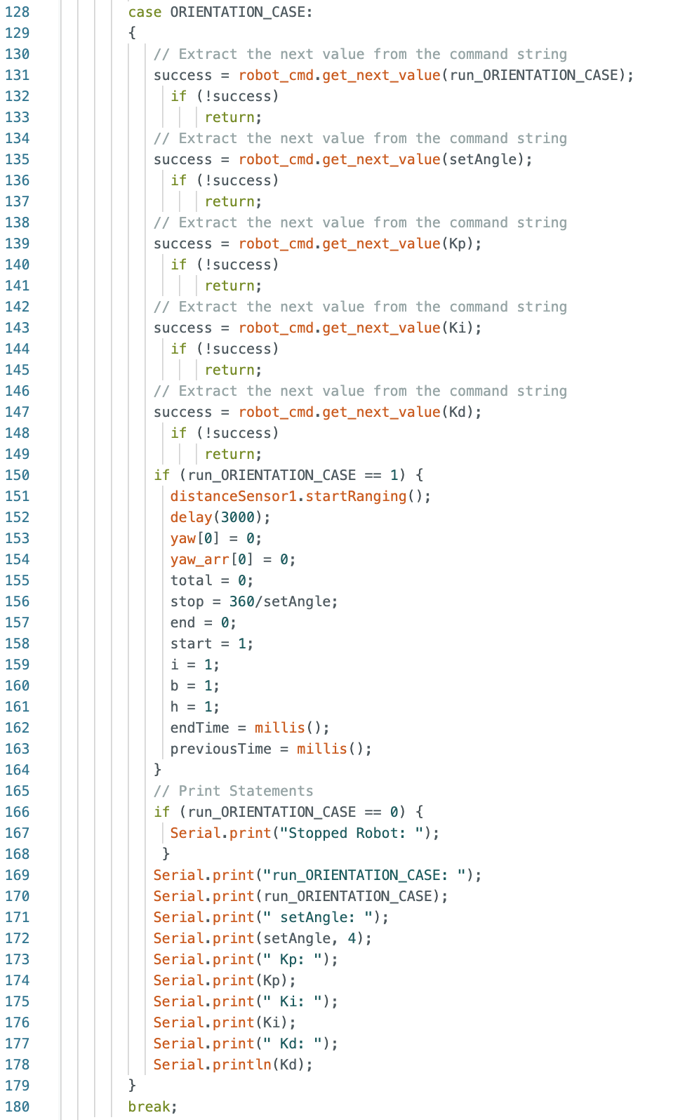
The Jupyter Notebook command and Arduino case to start the PID orientation controller are below. From testing I found that using a Kp value of 1, Ki value of 0 and Kd value of 0 worked to move the robot in 10 degree increments. Each time the PID orientation controller starts, yaw[0], yaw_arr[0], and the total are set to zero. In addition the stop variable is found. Graphs showing the changing yaw angles to confirm the PID controller works are found in the next section.

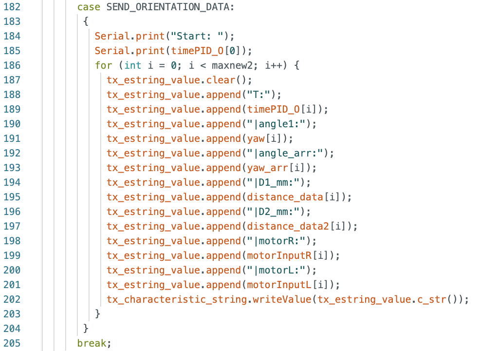
The Jupyter Notebook command and Arduino case to send the collected data are below.

Two videos of the robot turning are below. The robot roughly turns on axis. In the second video, the robot overshoots at some increments but is able to correct itself to the correct angle. The robot stays inside of one floor tile for the duration of the turn.
Turn 1:
Turn 2:
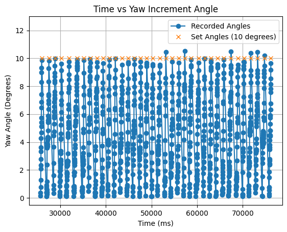
I plotted the values of yaw for each 10 degree increment. As can be seen in the below graph the PID controller works as expected. After yaw increases to 10 degrees, the value of yaw is reset to zero and then again increases to 10 degrees for the next increment. The slight variation in the final yaw value is due to the -0.5 to 0.5 degree tolerance.
The total angle values were found by adding each final yaw value (between 9.5 and 10.5 degrees) to a summation of all previous yaw values. The values and graph for an example turn are found below.

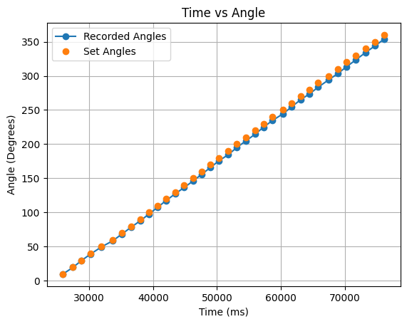
In the above graph as the turn progresses the angles remain accurate as the summation calculation is correct to the yaw reading of the robot, but the angles slightly vary from the ideal 360 degree turn values. To address this I also performed half turns from 0 to 180 degrees, and 180 to 360 degrees. The angle values and corresponding graphs can be found below:

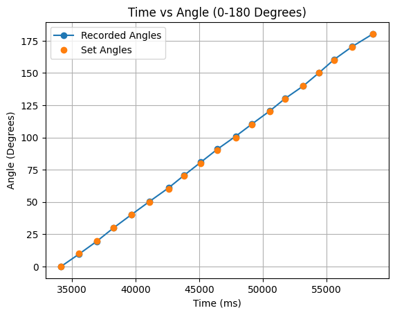

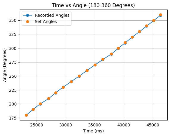
The half turns in the above graphs are more in line with the ideal angles. When testing the robot in the lab, I collected angle data for full turns and half turns.
There is no significant gyroscope drift in the IMU sensor because the robot resets the yaw value to zero after every 10 degree rotation. For a 360 degree rotation, the maximum error in the final angle value is -18 or +18 degrees (342 degrees or 378 degrees) if the yaw angle for every rotation is 9.5 degrees or 10.5 degrees respectively. For a 360 degree rotation, the average error in the final angle value is -9 or +9 degrees (351 degrees or 369 degrees) if the yaw angle for every rotation is 9.75 degrees or 10.25 degrees respectively. As noted previously, the final angle value for an example 360 degree turn is 353.859 degrees. A difference of (360 - 353.859) degrees = 6.141 degrees.
The robot turns roughly on axis, but the potential difference in the starting position and ending position may result in error for the distance measurements. Based on observing the motion of the robot the average error between the starting position and the ending position is 12mm, and the maximum acceptable error is 25mm. Due to friction, the robot might move off axis more for one rotation, while staying on axis for the next rotation. Assuming the robot moves off axis the same amount for each rotation, the average error in position for each rotation is 12mm/36 = 0.3333mm. The maximum error in position for each rotation is 25mm/36 = 0.6944mm.
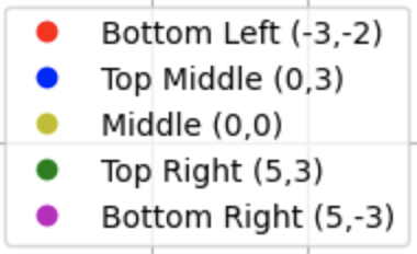
The robot was placed at each of the following points: (-3,-2), (0,0), (0,3), (5,3), and (5,-3). The image below shows each of the points in the lab.
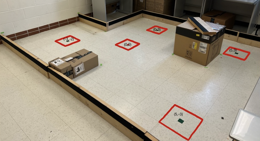
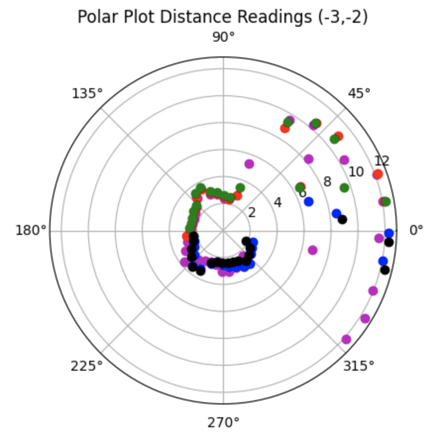
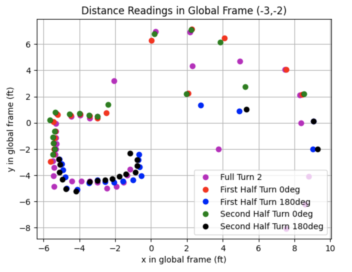
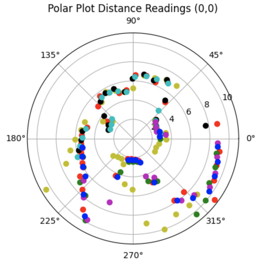
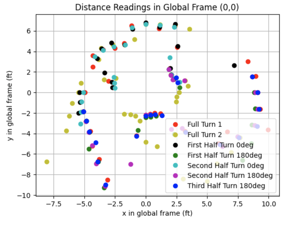
The distance was measured using the front ToF sensor between the left and right motor sides. The data collected was sent over Bluetooth to Jupyter Notebook to be plotted. The robot was started in the same orietation, facing the right side wall of the lab, for each full turn and each half turn starting at zero degrees. For half turns starting at 180 degrees, the robot started facing the left side wall. The range of potential angle values for each ideal 10 degree rotation is 9.5 degrees to 10.5 degrees. There is a -/+ 0.5 degree range for the robot to stop and collect a distance measurement. Due to the range of degree values, it can not be assumed that the robot will stop at exactly 10 degrees every time it rotates. This behaviour was desribed in the "Code for Orientation Control" section at the beginning of the lab report. The distance measurements can not be assumed to be spaced equally in angular space. To address this issue, I did not assume that the robot stopped at exactly 10 degrees for every rotation and instead recorded a "total" variable value that added the angle that the robot stopped at to the previously recorded stopping angle. This allowed me to plot the distance measurements with the correct recorded angles.
This section details the first attempt at collecting data at each point. The data collected for each point in the lab is plotted in the below graphs. For each point I plotted a polar graph and a global frame graph. The first two graphs show all of the data I collected for each point. The next two graphs show the data that I choose to keep when combining all of the global plots. In this section I noticed that the ToF sensor was pointed too downwards, resulting in a lot of noise in the middle of the plots. The noise resulted in the boundaries of the walls being hard to determine. After plotting this section I readjusted the ToF sensor to be pointed more upwards to avoid hitting the floor of the map.
All Data:
.png)
.png)
Partial Data:
.png)
.png)
All Data:
.png)
.png)
Partial Data:
.png)
.png)
All Data:
.png)
.png)
Partial Data:
.png)
.png)
All Data:
.png)
.png)
Partial Data:
.png)
.png)
All Data:
.png)
.png)
Partial Data:
.png)
.png)
The graph for the combined global frames can be found below.
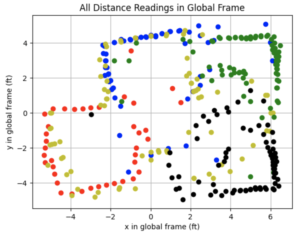
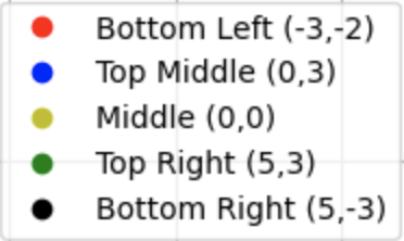
This section details the second attempt at collecting data at each point. The data collected for each point in the lab is plotted in the below graphs. I readjusted the ToF sensor to point more upwards before collecting the following data. This adjustement removed noise from inside the map region. The data collected for each point in the lab is plotted in the below graphs.
All Data:
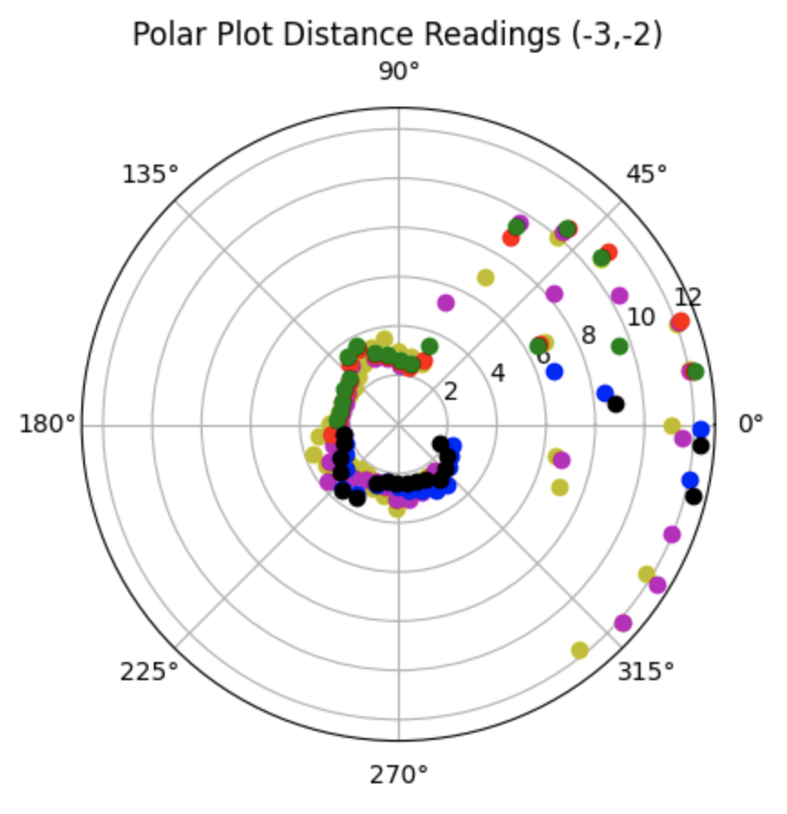
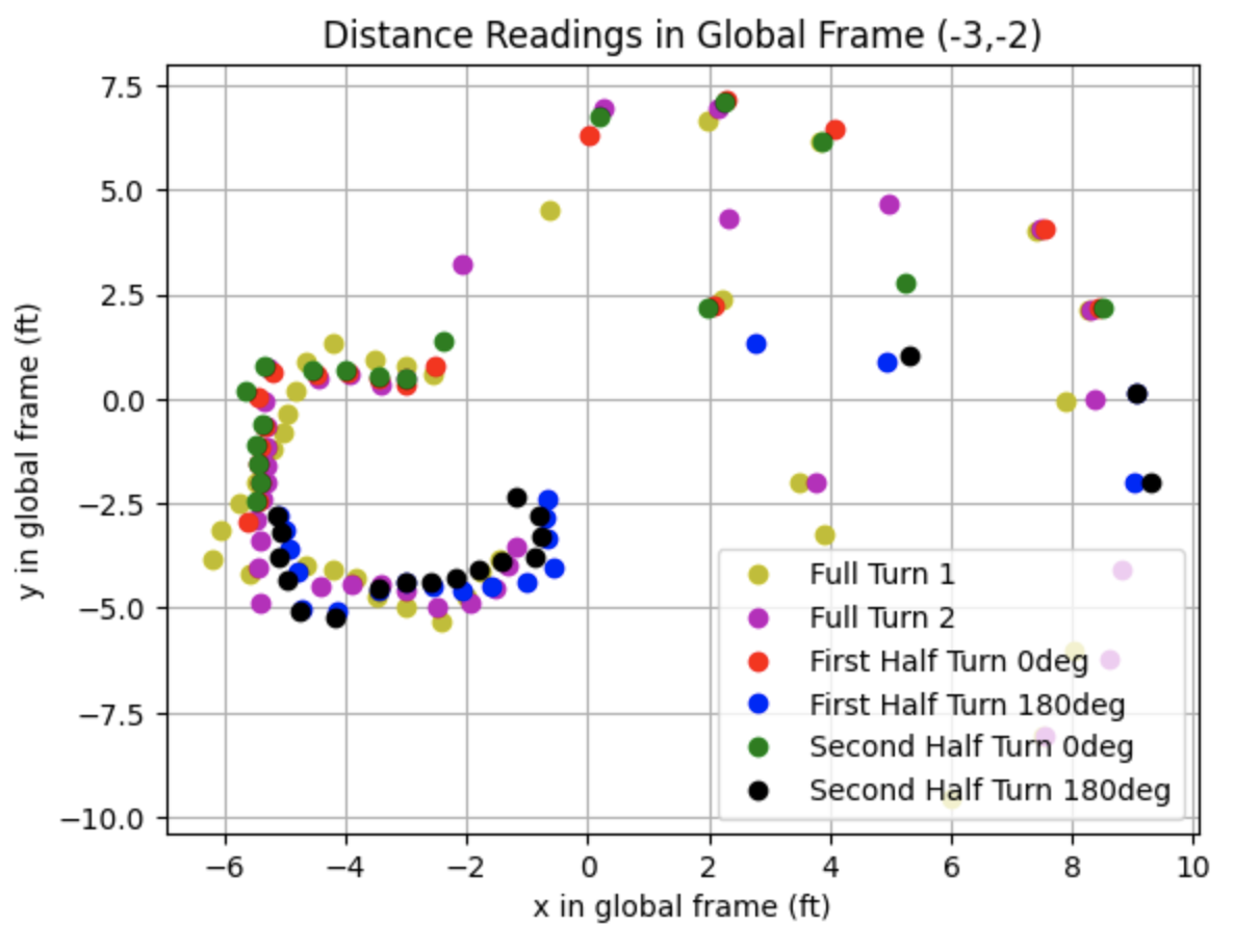
Partial Data:
All Data:
Partial Data:
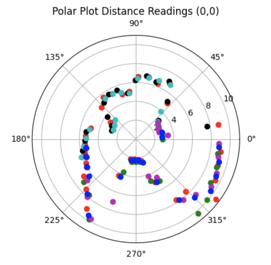
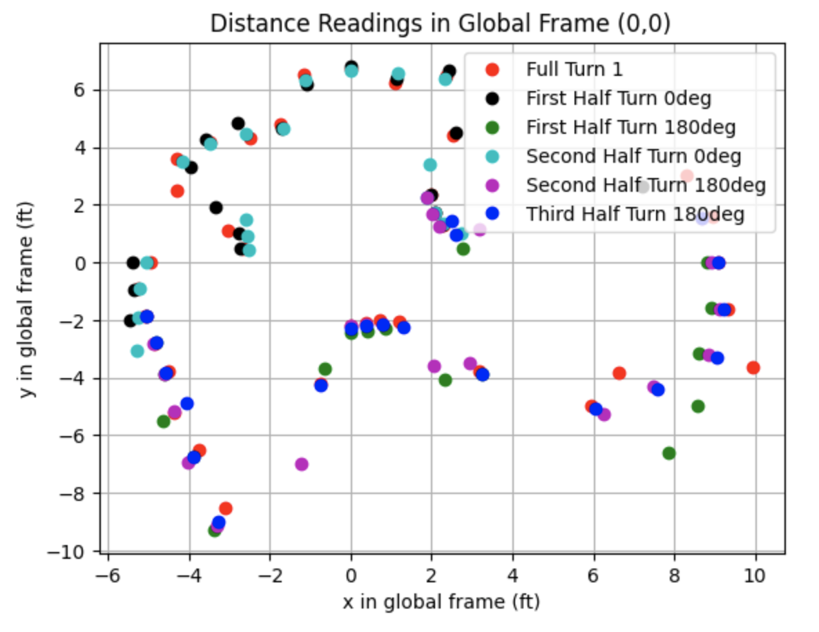
All Data:
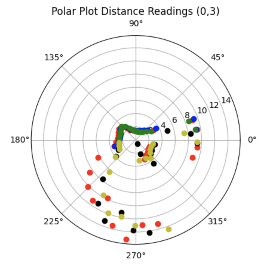
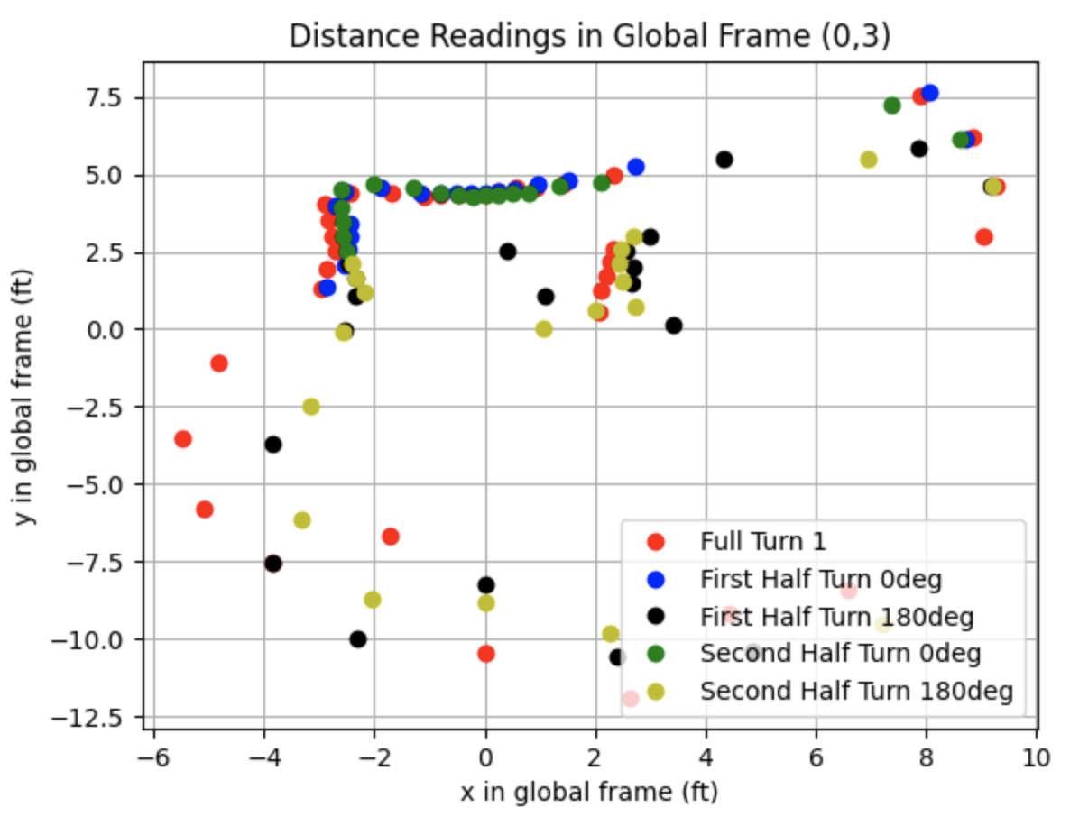
Partial Data:
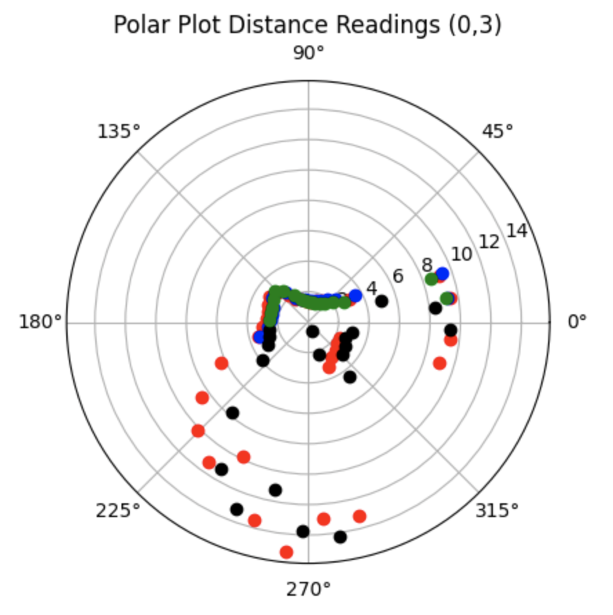
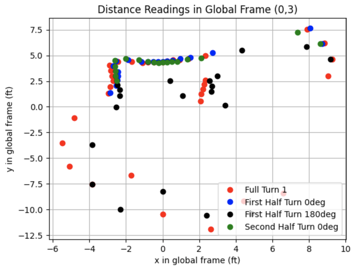
All Data:
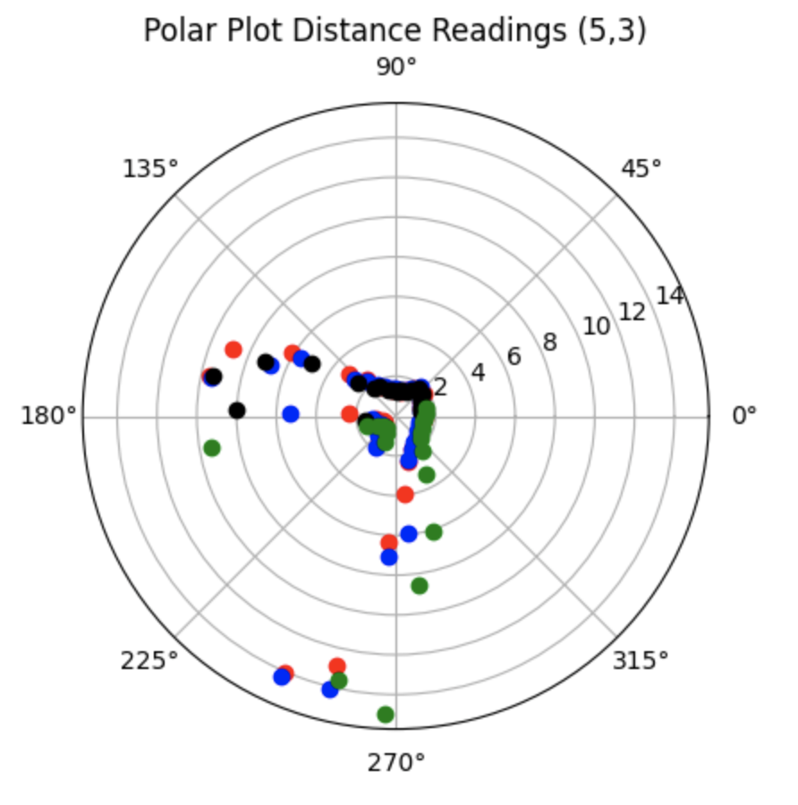
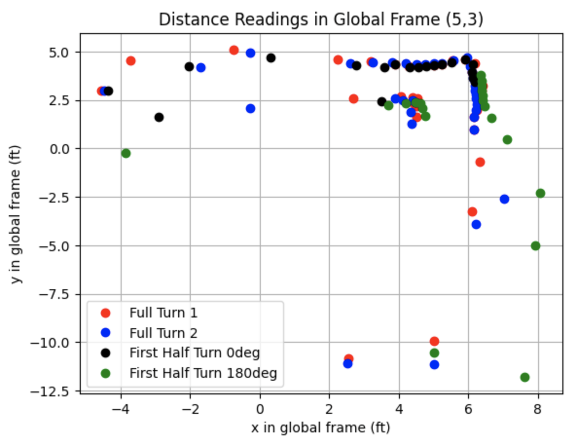
Partial Data:
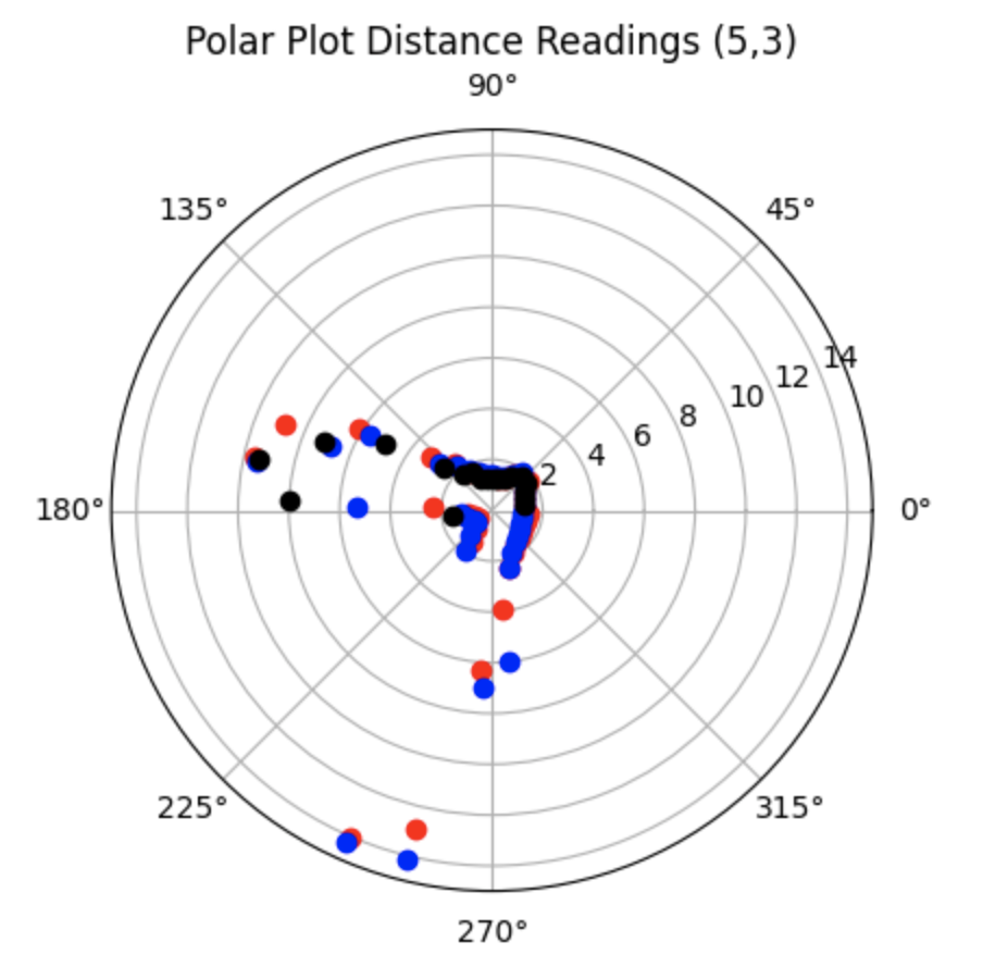
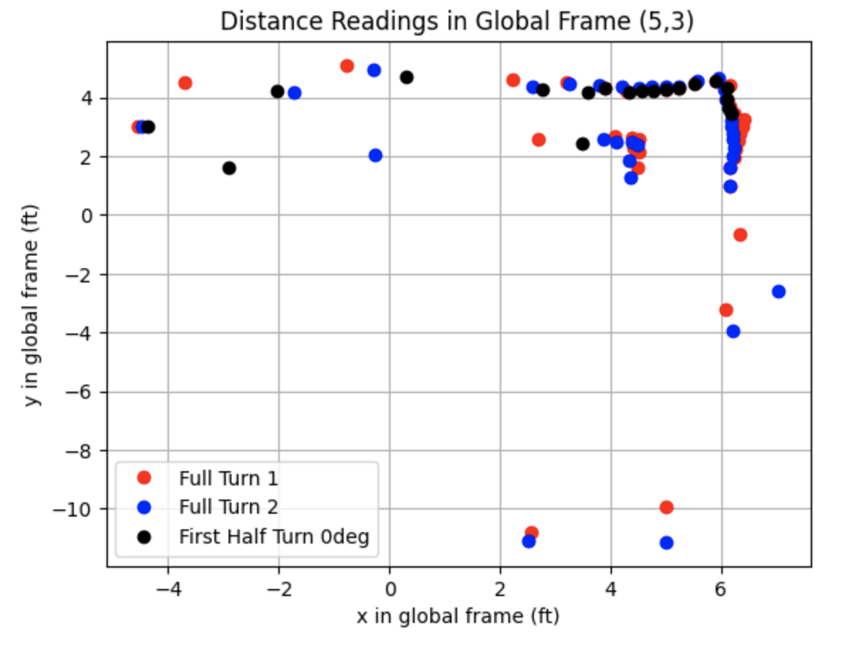
All Data:
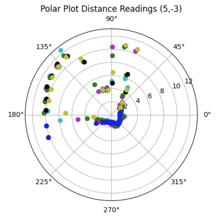
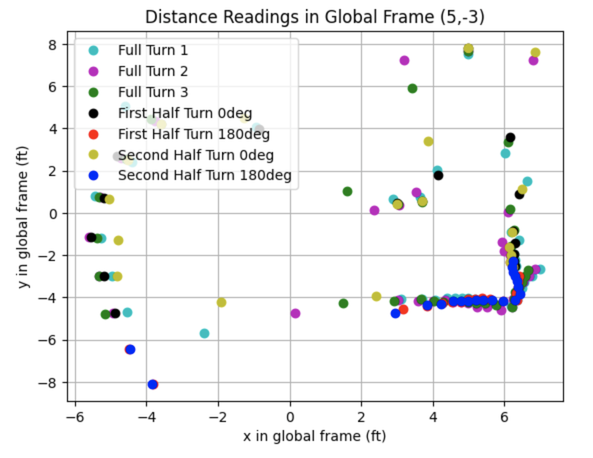
Partial Data:
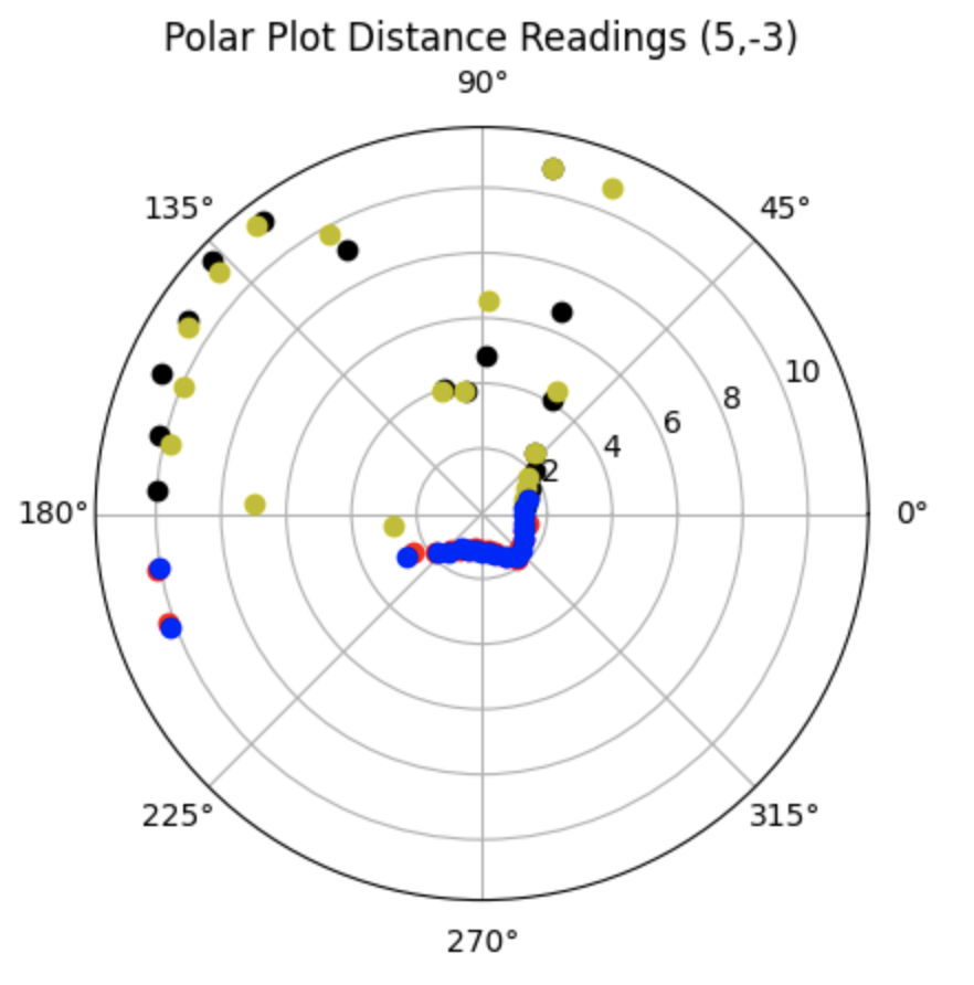
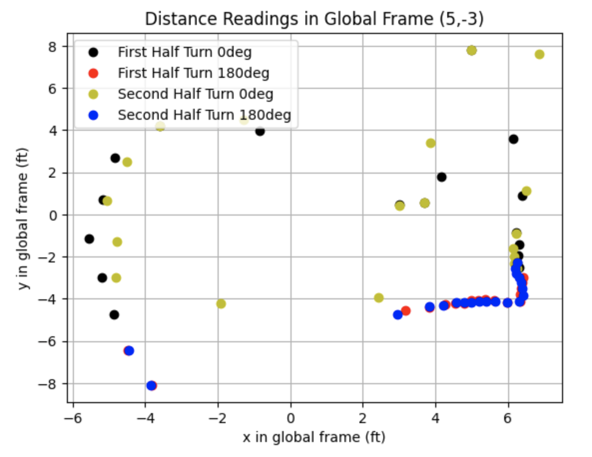
I plotted the distances in the global frame using the below transformation matrix. The transformation matrix converts the frame of the robot used to collect the sensor measurements into the global frame. The example below is for the point (-3,-2). The variable "theta" is the angle measurement in radians relative to the origin of the global frame and "dis" is the distance measurement. One ToF sensor between the left and right sides of the robot was used to collect distance data.
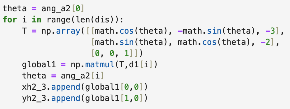
The code used to sort through the data is below.
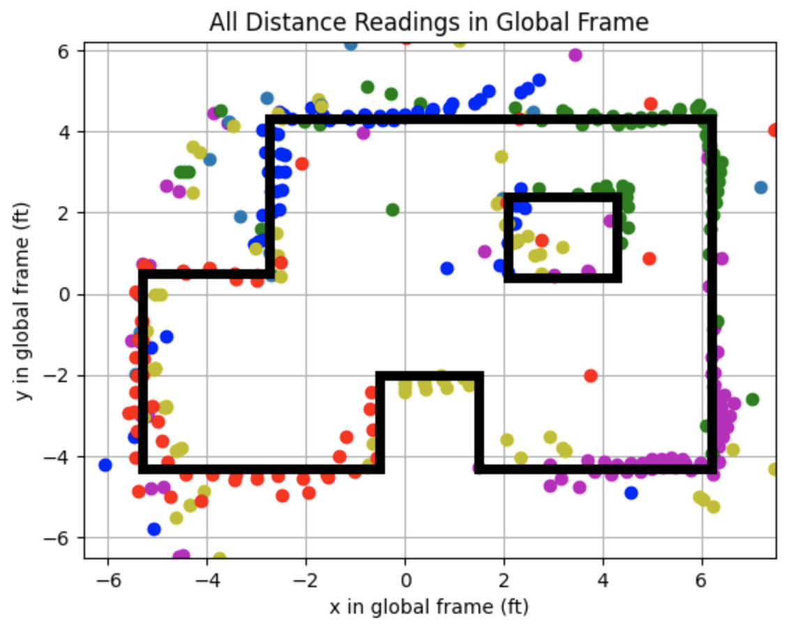
Below are the distance readings in the global frame.
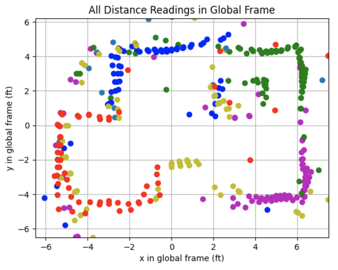
After plotting the above graph I plotted lines representing the walls of the map. The plot showing the line based map is below as well as the code used to plot each line.

Thank you to all of the TAs that answered my questions. I referenced the past lab reports of Liam Kain, Rafael Gottlieb, Larry Lu, Julian Prieto, and Ignacio Romo.
The objective of the lab is to implement a stunt on the robot using the knowledge gained from previous labs. Labs 5-8 detail PID, sensor fusion, and stunts. This lab is focused on using the ToF sensor and IMU sensor to drive the robot forward and then turn 180 degrees when the robot is within 3ft (914mm) of the wall. Task B: Orientation Control will be implemented on the robot.
The lab materials include a fully assembled robot with SparkFun RedBoard Artemis Nano, Pololu TOF Distance Sensors, and a IMU Sensor.
My inital approach to the orientation control stunt was to break down the stunt into three separate parts: driving towards the wall, turning, driving away from the wall. When driving straight towards the wall the robot uses PID control on the speed before slowing down and turning. The speed PID control function can be found below:
After the robot is within 3ft of the wall, PID control on orientation is used to turn the robot 180 degrees. The PID control value is determined by the yaw angle reading from the IMU sensor. If the PID control value is positive the wheels on the right side of the robot will move forwards and the wheels on the left side of the robot will move backwards. If the PID control value is negative the wheels on the right side of the robot will move backwards and the wheels on the left side of the robot will move forwards. The orientation PID control function can be found below:
The above two functions were called inside of the while loop. If the distance error is greater than zero, the speed PID control function is called. If the distance error is less than zero the orientation PID control function is called to turn the robot. The while loop can be found below:
Before implementing the final part of the task (driving away from the wall), I ran the above Arduino script. The inputs included a start/stop integer (1/0); a setDistance for the robot to start turning; and the Kp, Ki, and Kd PID values. While running the Arduino IDE code multiple times with different setDistance values (914mm-1300mm) and PID values, the robot did not perform in the expected manner. The robot would often either hit the wall or turn too late even when inputting larger setDistance values. In addition, the robot turned too slow whe inputting smaller Kp values (such as 0.5), or would spin multiple times when inputting larger Kp values (such as 2). Videos showing the behaviour of the robot are below:
The robot hits the wall before turning (setDistance = 915mm, Kp = 0.5):
The robot stops before hitting the wall, but turns too slowly during orientation control (setDistance = 1100mm, Kp = 0.5):
When a high value of 2 was used for Kp, the robot would spin too fast and not correct itself:
In addition, there were some bad runs that resulted in the robot turning towards the right immediately after starting the stunt due to the input PWM values:
After continuously testing the robot, I decided to write a new Arduino IDE script that only used orientation control. The robot runs towards the wall at a constant speed, and within the desired setDistance turns 180 degrees and moves away from the wall.
I first started working on implementing orientation control while the robot is driving forwards. Orientation control when the robot is driving forwards keeps the robot moving in a straight line. The robot is set to run at a base speed and PID control using the readings from the IMU correct the orientation of the robot to keep the robot at the starting yaw angle. Yaw was initially set to zero each time the case ran. Below are some videos of the robot being tested using orientation control at low speeds. Initially I tested the robot using the calibration factor of 1.1667 found in Lab 4, setting a base speed of 80 for pin 12 and 93 for pin 9. I found that setting each side of the robot to different speeds resulted in the robot moving towards the right or left as can be seen below:
I decided to set both pins to the same PWM value of 80 that resulted in the robot moving straight, as can be seen below:
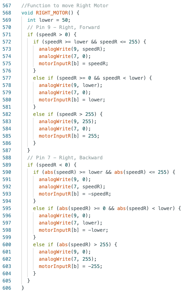
I added to the code for orientation control to make the robot turn 180 degress, rather than stopping as in the previous step. Initially yaw is set to zero and a base speed of 150 PWM was used for the motors on both sides of the robot. I tested various values for the setDistance and found that 1300mm allows the robot to recognize the wall with enough time to turn 180 degrees within 3ft and drive away from the wall. The Arduino code that runs inside the while loop is below. First the distance reading from the ToF sensor is found and used to calculate the error between the ToF sensor measurement and the setDistance. Then the yaw angle is found using the IMU and the error between the yaw reading and the desired setAngle is calculated. The yaw angle is used to find the orientation PID control value. If the distance error is less than zero (robot is past 1300mm) and the setAngle equals 0, the setAngle will be changed to 180. If the orietation error is greater than or equal to -3, or less than or equal to 3, the left and right side motors will be set to the base speed. If the previous condition is not met, the left side motor will be set to the base speed minus the PID control value and the right side motor will be set to the base speed added to the PID control value. The code inside the while loop is found below:
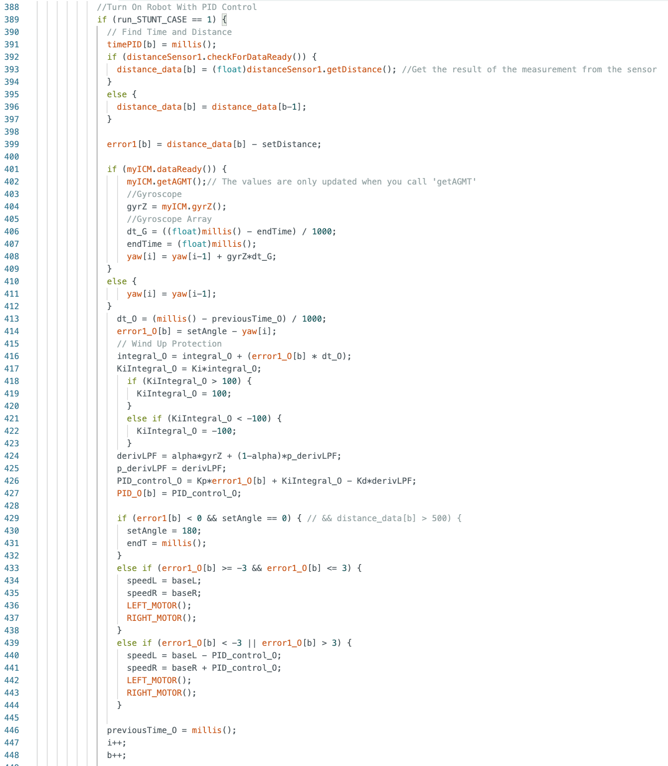
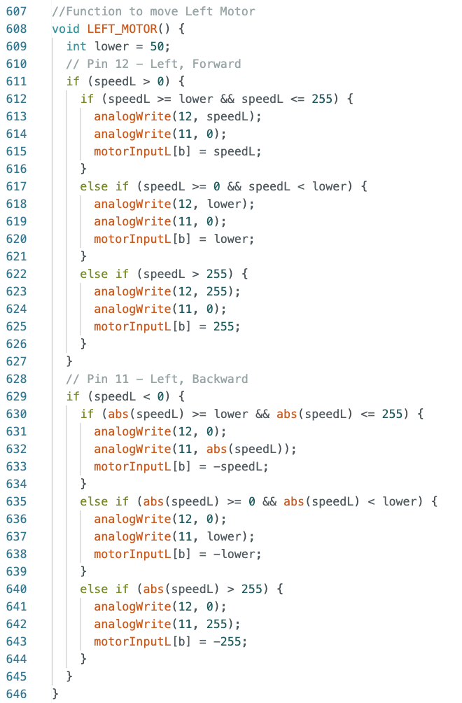
The RIGHT_MOTOR and LEFT_MOTOR functions are below:
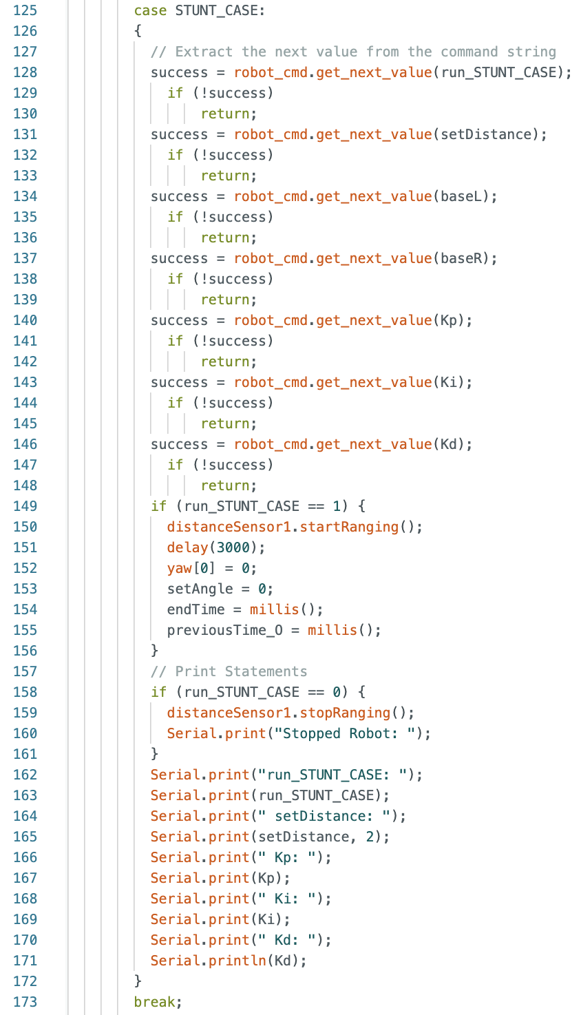
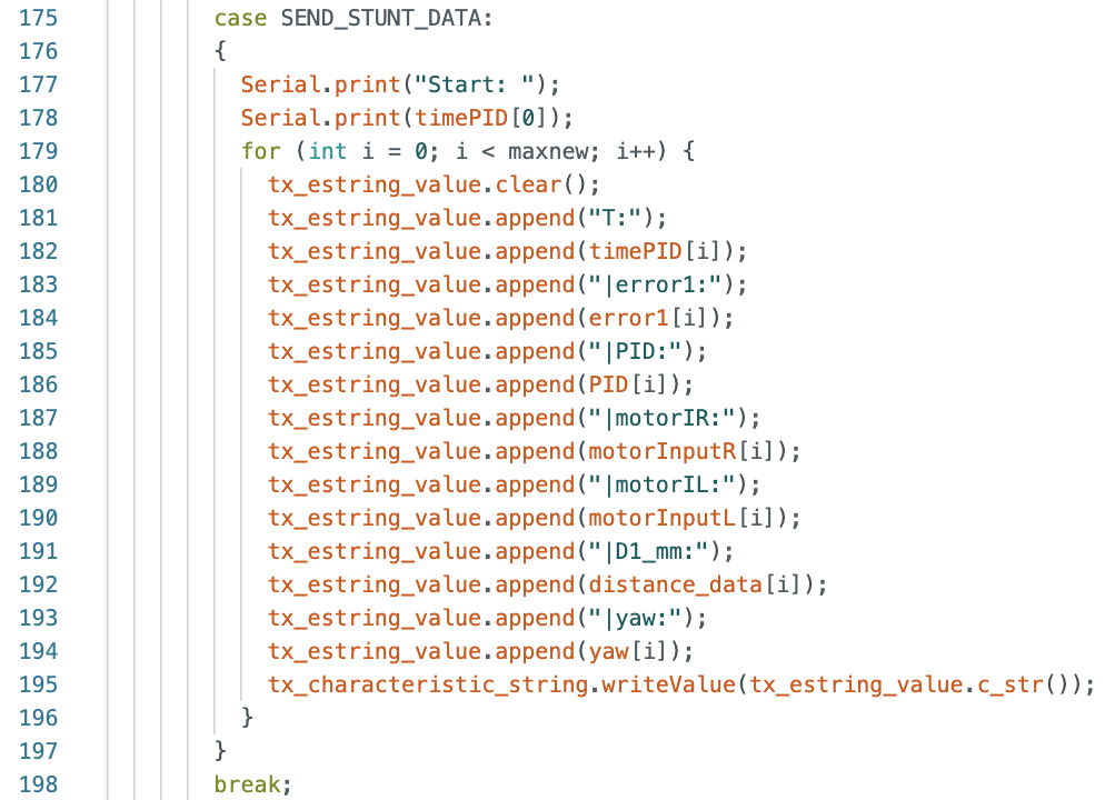
The Arduino cases and Jupyter Notebook commands for STUNT_CASE and SEND_STUNT_DATA are below. The ToF distance sensor starts ranging, yaw is set to zero, endTime is found, and previousTime_0 is found when the run_STUNT_CASE is set to 1.


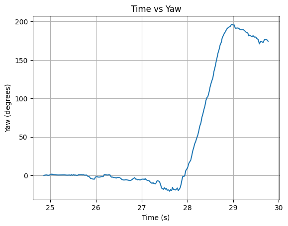
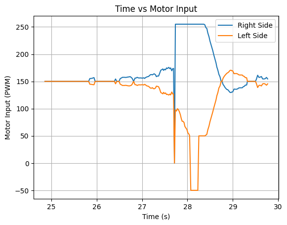
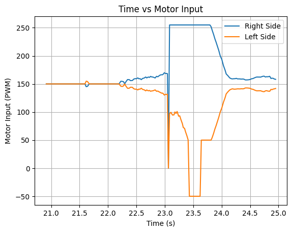
The three working stunt videos are found below. The base speed is 150 for both motors, setDistance is 1300mm, Kp = 1.25, Ki = 0.01, and Kd = 0.05. The stunt takes around 4 seconds to run.
Below are graphs showing the ToF distance readings, yaw angles, and motor input values. The graphs show that the robot turns before hitting the wall.
Run 1:
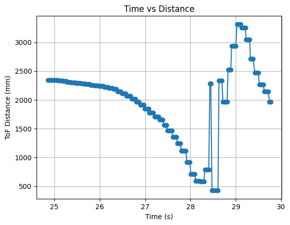
Run 2:
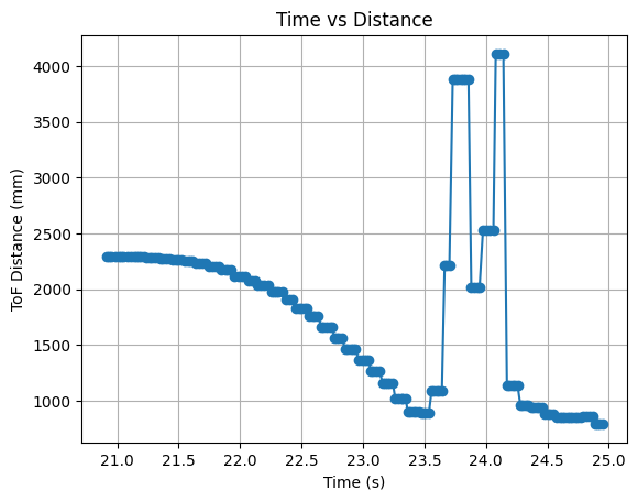
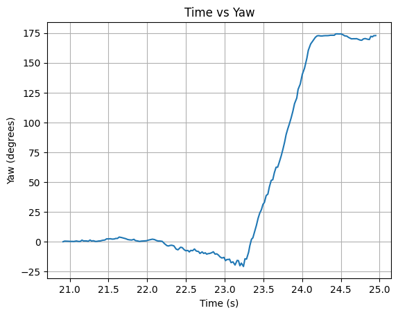
The below video shows the serial monitor outputs for the code used to run the stunt.
Thank you to all of the TAs that answered my questions. I referenced the past lab reports of Liam Kain, Rafael Gottlieb, Larry Lu, Julian Prieto, and Ignacio Romo.
I implemented the Kalman Filter on the robot for extra credit. To complete this task I needed to install the Basic Linear Algebra Library on Arduino IDE. To implement the Kalman Filter I first created two new cases in Arduino IDE: KF_DATA and SEND_KF_DATA. These cases are similar to the cases used to start/stop the PID controller and send PID controller data, but I added array's for Kalman Filter time (KF_Time) and the Kalman filter distance (mu_Store). I added a delay in KF_CASE before running the while loop. When I was testing the filter I was repeatedly starting with distances of 0mm. The delay after the ToF distance sensor starts ranging reduces the amount of 0mm distance readings when starting the filter. The Arduino cases and Jupyter Notebook commands can be found below:

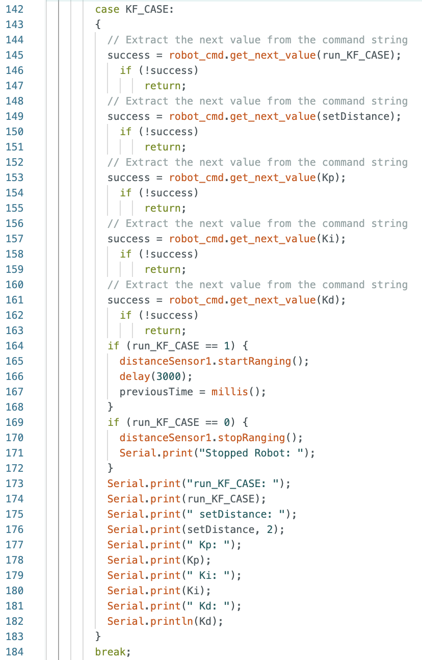

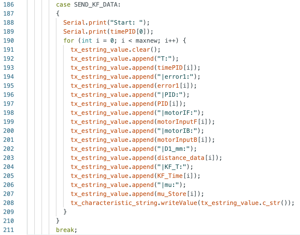
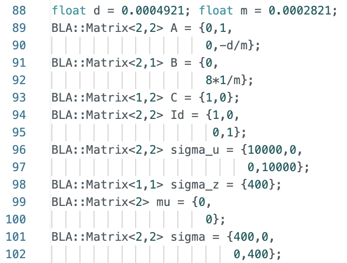
After creating the cases for the Kalman Filter, I then started working on writing a Kalman Filter function in Arduino IDE. The final initialization of the matrices is below:
The first function that I wrote for the lab was the function Kalman_Filter() that is called from inside the larger while loop. To perform this task, I referenced the Jupyter Notebook code I wrote for Lab 7 and modified the code for the Arduino IDE syntax. The function can be seen below:
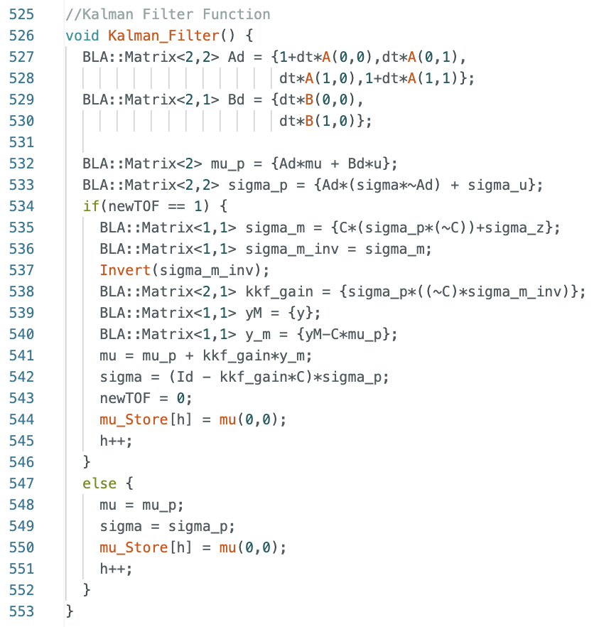
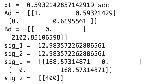
The Ad (discritized A) and Bd (discritized B) matrices are updated each time the Kalman Filter is called to use the most recent dt value. I printed the dt (time difference) values to the Serial Monitor and observed that the dt values slightly varied each time the while loop ran. The variable dt is how fast the while loop runs and ranged from around 10ms to 25ms. After finding Ad and Bd, mu_p and sigma_p are calculated. The if statement of the filter is the update step and runs when there is a new TOF sensor reading (newTOF == 1). The else statement is the prediction step and assigns the mu_p value to mu and the sigma_p value to sigma. During both steps the first value for mu is stored in the array mu_Store.
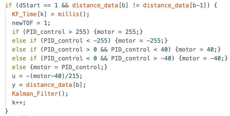
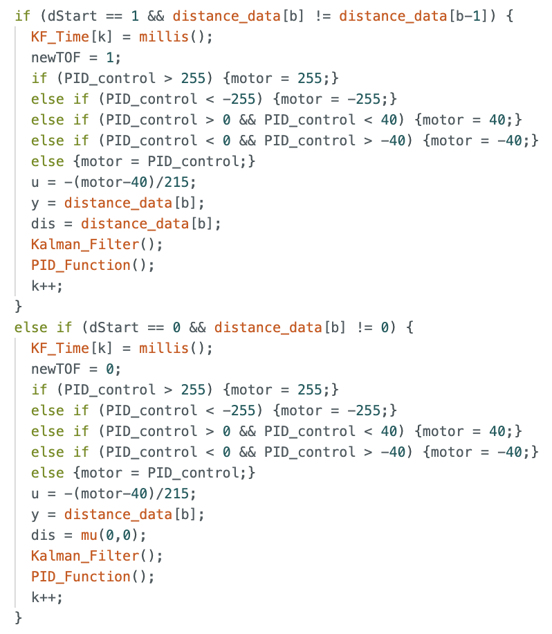
I started working on the calling the Kalman Filter from inside the while loop by modifying the script for my PID controller. After finding the ToF sensor readings and running the PID controller within the larger while loop, I added an if statement inside the loop to call the Kalman Filter to find the update values. The if statement runs if dStart == 1 and if the currect distance value is not equal to the previous distance value. The variable dStart is set to 1 if the new ToF sensor distance is not the same value as the previous sensor distance. If the current distance reading is the same as the previous distance reading dStart is set to 0. The if statement to call the update of the Kalman Filter is below:
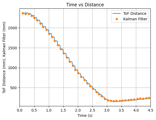
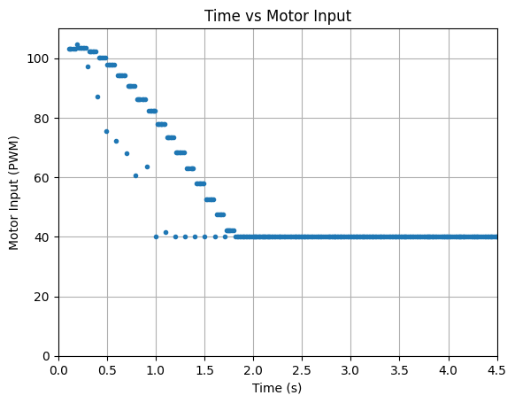
The PID controller was run using values of Kp = 0.05, Ki = 0.0000008, and Kd = 0.5. A test run showing the plotted ToF data and the Kalman Filter updates is shown below. It can be seen that the Kalman Filter updates align with each new reading of the ToF sensor.
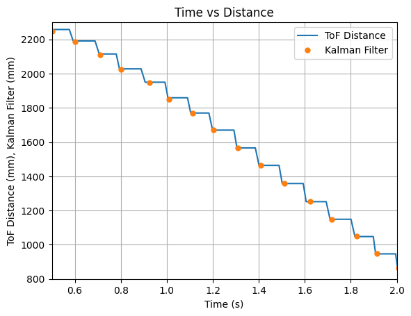
The video below shows the Serial Monitor outputs for the ToF distance readings and the update values:
The full while loop code for this section is below:
The FORWARD() Function that was used previously for PID control is below:
The BACKWARD() Function that was used previously for PID control is below:
After successfully implemeting the update step of the Kalman Filter, I started working on the prediction step.
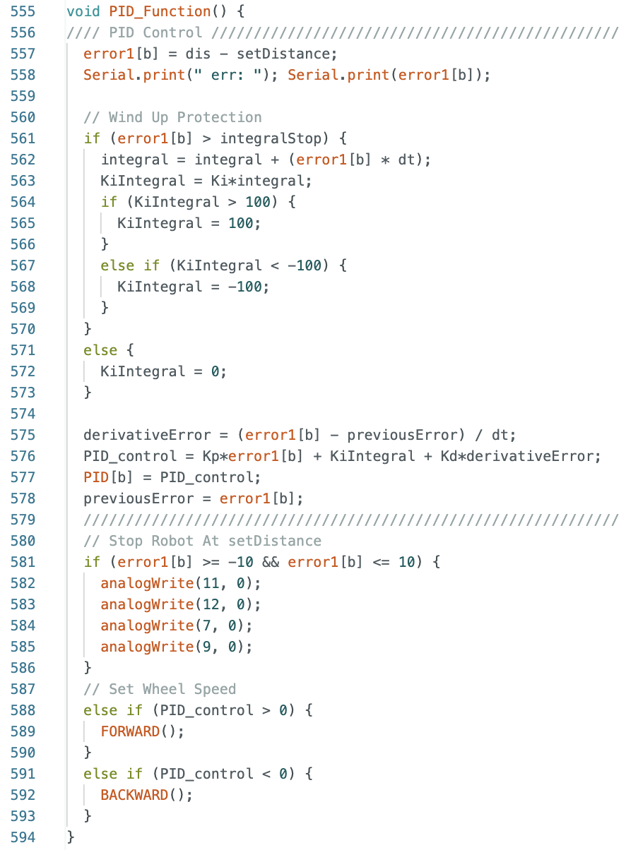
I started the next step by removing the PID control from the larger while loop and creating a separate function called PID_Function(). A separate function for PID control allowed for me to more easily switch the order to performing the Kalman Filter before the PID controller. Previously the PID controller used the ToF sensor measurements every time the loop ran. In the new iteration of the code, if the update step of the filter runs, the distance measurement used will be the ToF sensor reading. If the prediction step runs the most current value of mu will be used in the PID controller. The if and else statements for the update and prediction steps are shown below. The variable dis is the distance measurement used in the PID controller. The u value for the Kalman Filter was calculated the same as in Jupyter Notebook using the PID control values.
The PID_Function is below:
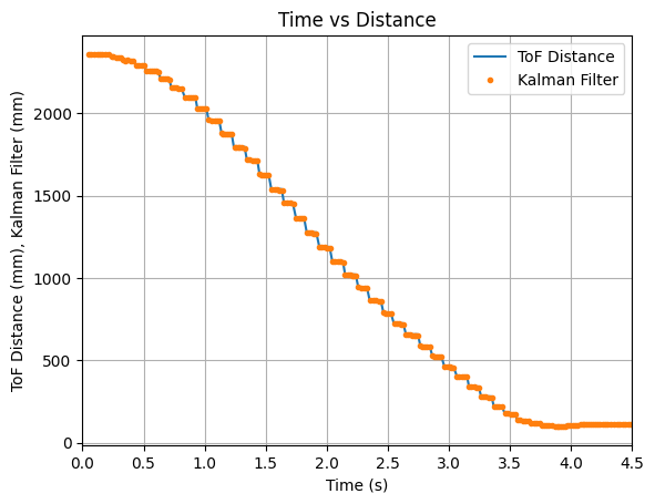
The PID controller was run using the same Kp, Ki, and Kd values as the previous section. An initial test run showing the plotted ToF data and the Kalman Filter updates is shown below. The graphs show that the filter is predicting distances between ToF readings, but the predicted values do not follow the trend of the data towards the next update value.
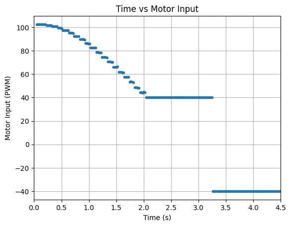
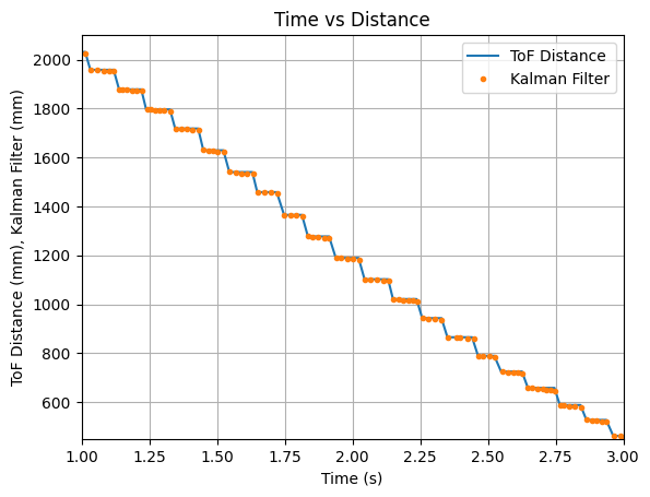
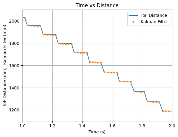
To address the above issue, I multiplied the B matrix by 3 and again tested the robot. The graphs below show that multiplying matrix B by 3 did not significantly change the predicted values.
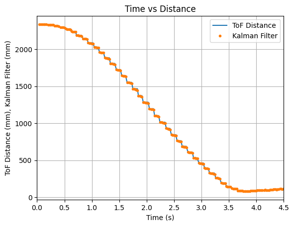
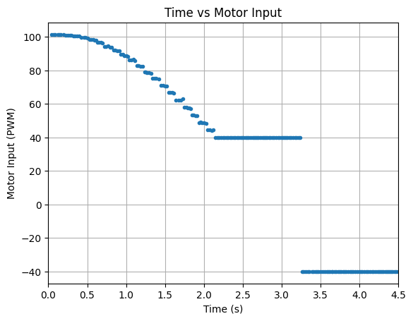
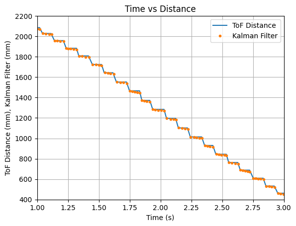
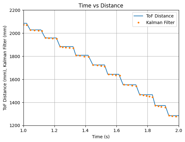
I then multiplied the B matrix by 6 and achieved the below results. The predicted values trend downwards, but still do not reach the update values.
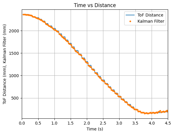
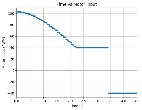
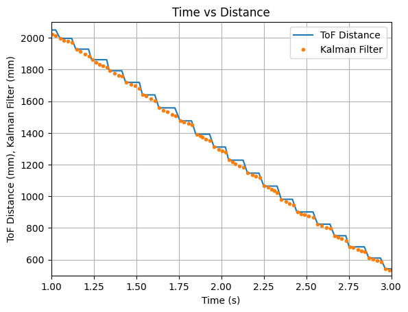
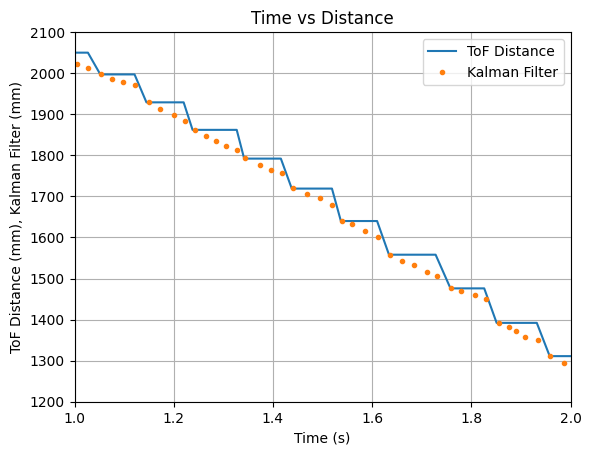
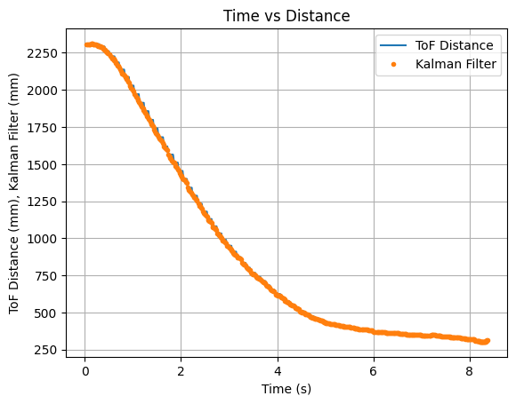
Throughout more testing, I determined that a good value to multuiply the B matrix with is 8. The Kalman Filter updates align with each new reading of the ToF sensor and the prediction values follow the trend of the data. Below are two sets of graphs showing data that was recorded after the B matrix was multiplied by 8. Needing to multiply the B matrix by 8 indicates that the value found for m during the Jupyter Lab simulation does not work as well when implementing the Kalman Filter on the robot.
Test 1:
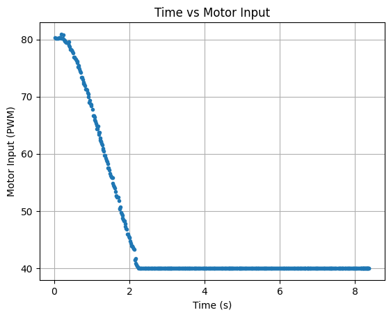
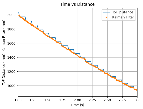
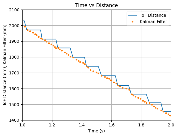
Test 2:
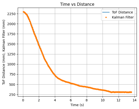
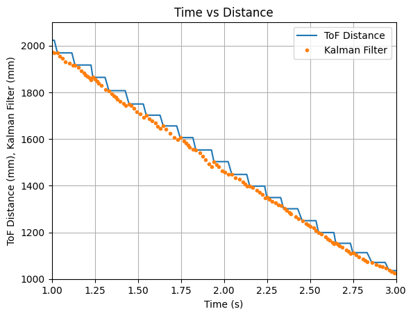
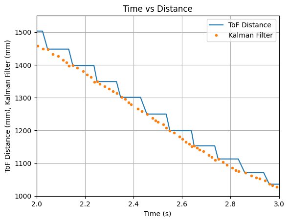
In addition during testing, I accidentally set the robot to a higher speed than necessary and the robot ran into multiple walls and did not always travel in a straight line for the below run. I decided to run the collected data through the Kalman Filter to see the outcome. The graphs below show that the update values and some of the predicted values align with the recorded ToF data. The Kalman Filter is able to update to the correct ToF value, even during somewhat random running conditions.
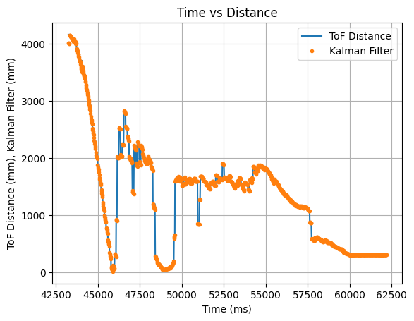
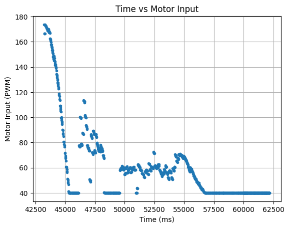
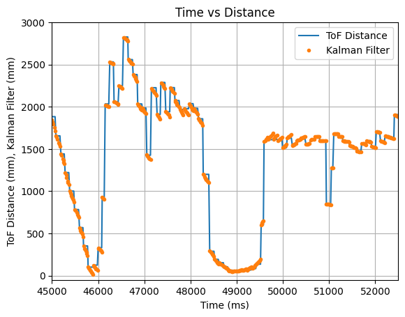
The video below shows the Serial Monitor outputs for the ToF distance readings and the update values:
Below is an example run of the Kalman Filter on the robot:
The full while loop code for this section is below:
While I was implementing the Kalman Filter onto the robot I was able to work through most of the debugging in an efficient manner. One mistake that I made early during implementation was not converting dt to seconds which caused my predicted values to drastically increase or decrease. Initially I thought that there was a problem with my sigma values and spent time changing the sigma values to see if there was any change. This did not work and I discovered the issue with dt during office hours.
Thank you to all of the TAs that answered my questions. I referenced the past lab reports of Liam Kain, Rafael Gottlieb, Larry Lu, Julian Prieto, and Ignacio Romo.
The objective of the lab is to gain experience implementing Kalman Filters. Labs 5-8 detail PID, sensor fusion, and stunts. This lab is focused on using a Kalman Filter to predict ToF sensor distance readings of the robot. The code from Lab 5: Linear PID Control will be used to gather data, having the robot speed towards a wall and stop 1ft in front of the wall. A Kalman Filter will be implemented in Jupyter Notebook using the collected data.
The lab materials include:
A Kalman Filter uses a state space model to predict the location (distance from the wall) of the robot. The location of the robot is predicted and then updated using the ToF sensor reading. The prediction and update steps from Lecture 13 are below:
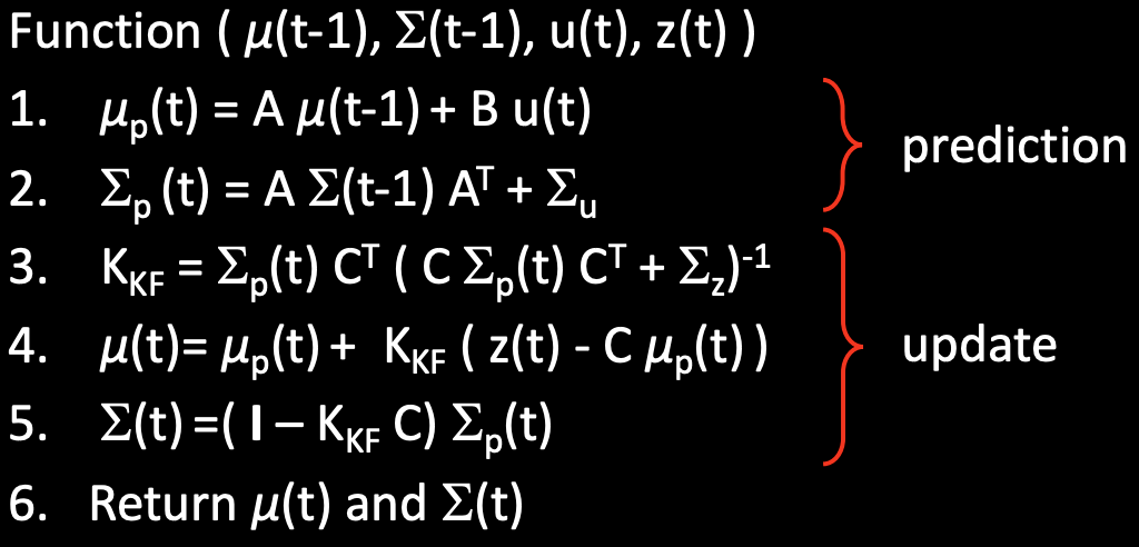
The state space model is used to find the A, B, and C matrices. The state space model for the robot from Lecture 13 is below. The model uses drag (d) and momentum (m) to form the A and B matrices. The two states are the location of the robot and the robots velocity.
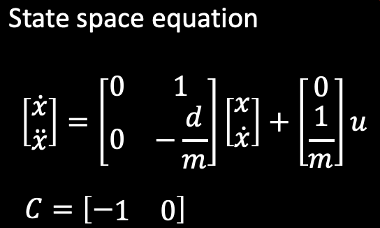
The first part of the lab is estimating the drag and momentum of the robot using steady state velocity. One difference from the lecture slides is that for this lab the C matrix will be C = [1 0]
The drag and momentum for the A and B matrices are estimated using a step response. The robot drives towards a wall at a constant input motor speed. The ToF sensor distance measurements and motor input values are recorded. Velocity is calculated and plotted along with the 90% rise time. The data is used to determine the drag and momentum and build the state space model of the system.
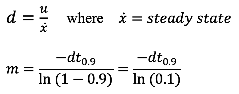
The equations for drag and momentum are below:
The step response u(t) was chosen to be a PWM value of 165. The step response is 64.71% of the maximum u PWM value of 255. I choose a PWM value of 165 as it was the fastest the robot could move while still moving straight for a distance of around 6.5ft. I collected time, ToF distance readings, and used these readings to calculated the velocity. To ensure that the step time was long enough for the robot to reach steady state, I ran the test multiple times. The results from the first test are below:
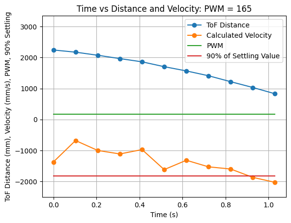
Looking at the results from the first test it can be seen that the maximum velocity reached is just over -2000mm/s. This velocity was only reached once. To confirm the steady state speed, the test was run again and the following results were plotted:
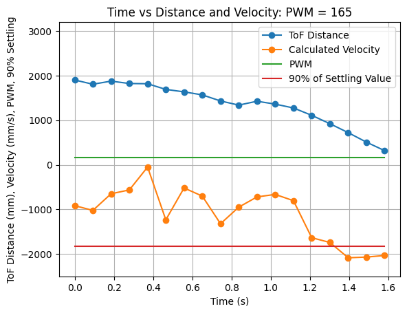
From the above graph it can be seen that the steady state velocity is just over -2000mm/s, or more specifically -2031.91mm/s. Using a 90% rise time a line on the above graph was plotted showing 90% of the settling value. This value is (-2031.91mm/s * 0.9) = -1828.72mm/s. The 90% rise time can be determined from the graph as 1.32s. The steady state velocity is used to find the drag. The drag and rise time are used to find the momentum. The calculations to find drag (d) and momentum (m) are found below:
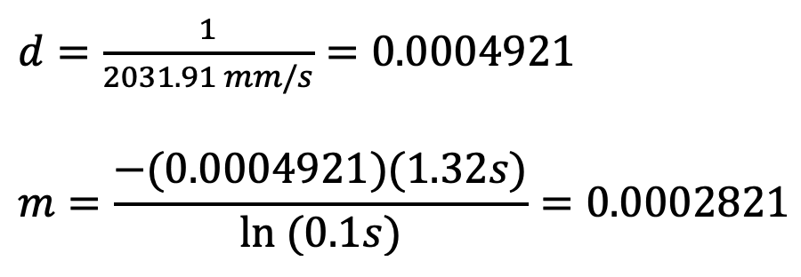
Calculated: d = 0.0004921 and m = 0.0002821
Drag is inversly proportional to the speed of the robot and affects how much the system reacts to changes in u. Momentum relates to how much effort is needed to change the velocity. Higher momentum signifies that more effort needs to be exerted to change the velocity, whereas lower momentum signifies that less effort needs to be exerted to change the velocity.
The collected data array's from all trials were stored in Jupyter Notebook in case the data needed to be used in the future. The code to find the steady state velocity can be found here: Max Speed Code
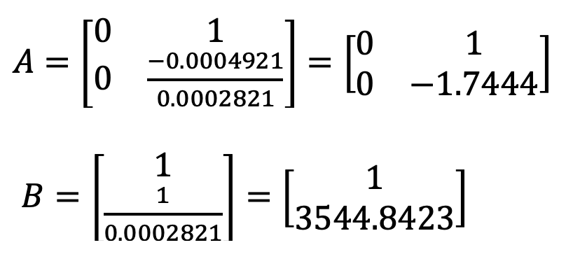
The A and B matrices were computed using the calculated values for d and m. From the state space equation the A and B matrices are:

The A and B matrices were calculated as seen below:
The discritized A and B matrices are calculated using the following method from Lecture 13:
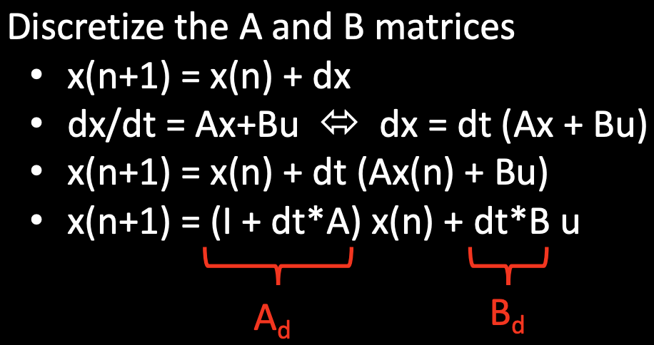
Initially, the sampling time for the discritized Ad and Bd matrices was calculated by subtracting the first time stamp from the second time stamp. After looking closely at the data, the sampling time between each time step was slightly different. I changed the calculation for Delta_T to be an average of all of the sampling time differences. The Delta_T was recalculated for each new dataset that I graphed. Below is an example calculation of the discritized Ad and Bd matrices, using the found sampling time of 0.008s for the PID loop in Lab 5. This dt is how fast the PID control loop is running.

The provided code in the lab report as well as my method of finding Delta_T was used to implement the calculation in Python as seen below:
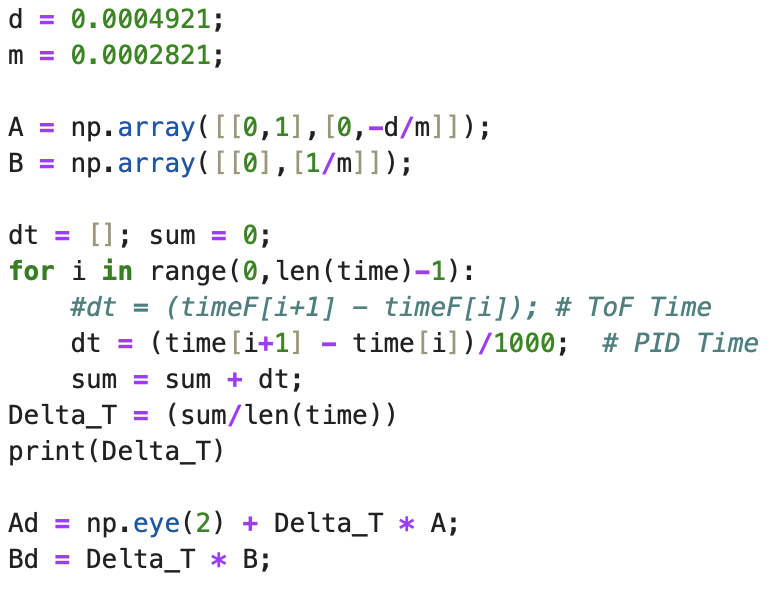
There are two different time array's. One method of finding Delta_T uses the time array of the PID controller (array: time). This method was for the 5000 level task, resulting in a faster frequecy than the frequency found for the ToF readings (array: timeF). In between ToF readings the prediction step of the Kalman Filter estimates the state of the robot.
The previously used code that does not calculate the average sampling time to find Ad and Bd can be found here: Previous Ad Bd Code
The C matrix for the state space is C = [1 0]. C is an m x n matrix where m is the number of states measured (1, ToF sensor distance) and n is the dimensions of the state space (2, ToF distance and velocity). The initial state is the first distance measurement and a velocity of 0 as the robot is not yet moving. The positive distance from the wall was measured.
Below is the Python code to establish the C matrix and initialize the state vector for the ToF distance measurements.

The process noise and the sensor noise covariance matrices need to be specified for the Kalman Filter to work well. Sigma_3 was initialized as 20. This value was determined from slide 35 in Lecture 13 as well as the ToF sensor datasheet. Sigma_Z represents the mistrust in the sensor readings. The ToF sensor has a ranging error of +/- 20mm in ambient and dark lighting.
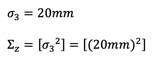

Sigma_1 and sigma_2 were initialized using the calculation found on slide 35 of Lecture 13. Sigma_U represents the mistrust in the Kalman Filter model. Sigma_1 is the relationship between the ToF distance reading and the model predictions. Sigma_2 is the relationship between the velocity and the model predictions.
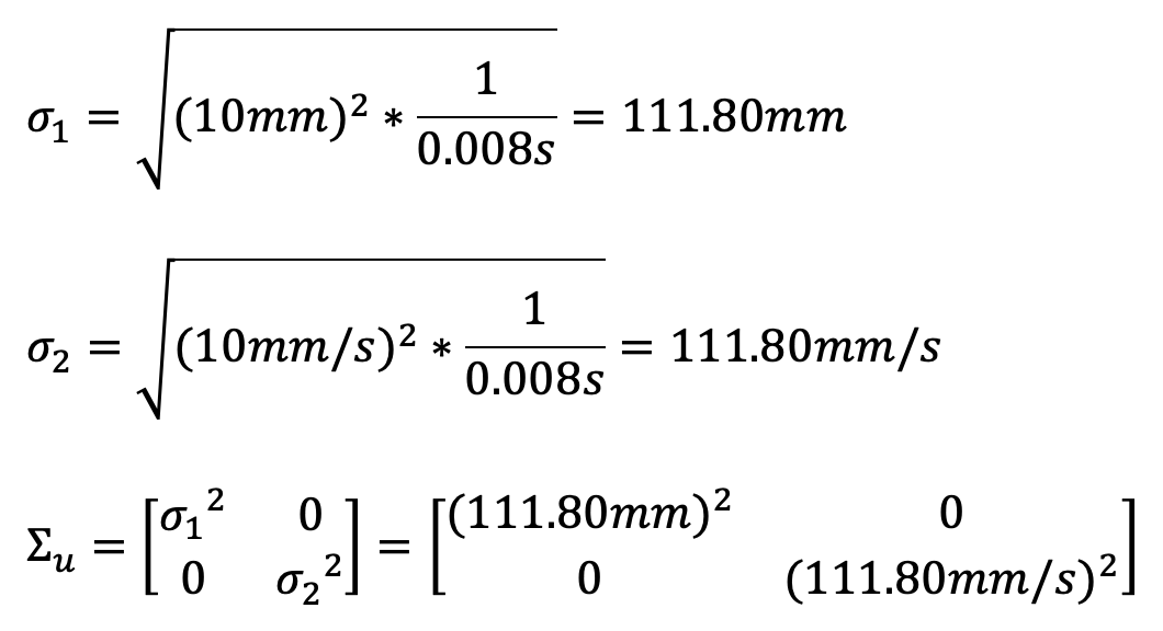
In Jupyter Notebook, I calculated the sigma values for each dataset as shown in the below code. The initiallized sigma had a value of 20 for sigma_1 and 5 for sigma_2 as the robot is not moving initially.
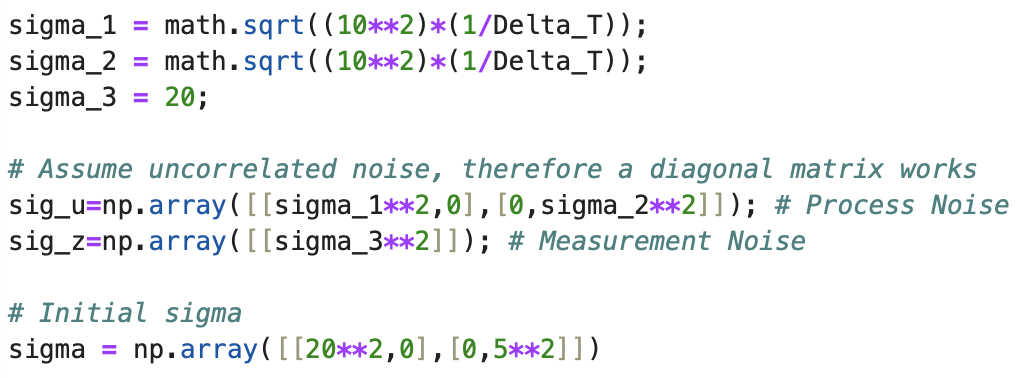
The sigma values were altered as needed for each dataset.
The below section includes the 5000 level task to use a faster frequency and use the Kalman Filter prediction step to estimate the state of the car, as well as the same data graphed without the prediction step for comparison. To write the below code I went to office hours to ask questions and looked at all of the lab reports for the TAs.
The below code for the Kalman Filter function was provided in the lab instructions and implemented in Jupyter Notebook.
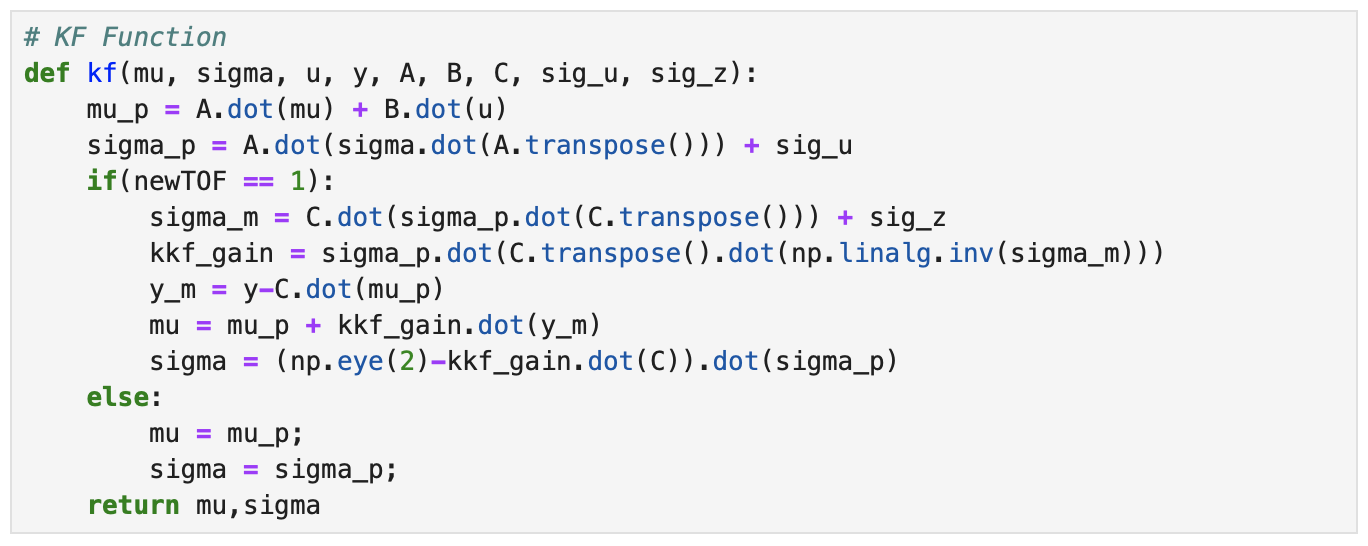
The first two lines finding mu_p and sigma_p are the prediction step of the Kalman Filter. If there is no new ToF sensor reading, then the returned mu and sigma will be equal to what is found during the prediction step. Within the if statement there is the update step of the Kalman Filter that runs every time there is a new ToF reading. The current state is mu, the uncertainty is sigma, the motor input values are u, and the distance readings are y.
To loop through each time step the below code was used.
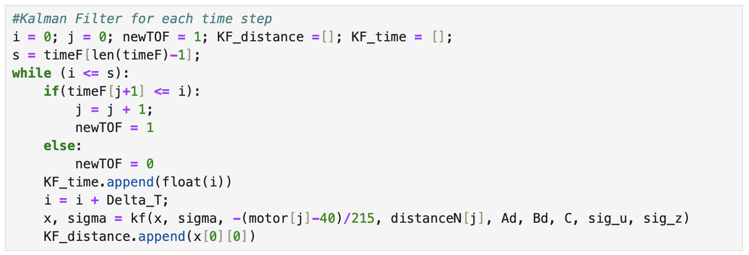
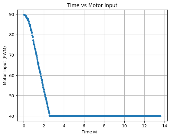
The while loop determines how many times the Kalman Filter runs. How many times the while loop runs depends on the the second to last time step for a ToF sensor reading and the value of Delta_T. If the value of the ToF time array is less than or equal to the value of the index, i, then the value of newTOF will be set to 1 and the update step of the Kalman Filter will run. If the value of the ToF time array is not less than or equal to the value of the index, i, then the value of newTOF will be set to 0 and only the prediction step of the Kalman Filter will run. The index i is updated by adding Delta_T each time the while loop runs and the value of i is appended to the array KF_time to plot the Kalman Filter. After i is updated, the Kalman Filter function is called and then the output distance (x) is appended to the KF_distance array to later be plotted. The u input was the negative value of 40 subtracted from the motor array storing PWM values, divided by 215 (the upper bound of 255 minus the lower limit of 40). The lower limit PWM value is 40. In this model if the motor input value is 40 then the value for u is zero (-(40-40)/215).
Throughout the lab report I discuss the parameters used to modify the Kalman Filter and in the section below I discuss how the parameters are modified to better fit the Kalman Filter to the ToF distance data. To summarize, the parameters include the sampling time (Delta_T), drag (d), momentum (m), and sigma values including Sigma_1, Sigma_2, and Sigma_3. The sigma values are used to find the covariance matrices: Sigma_U and Sigma_Z. Sigma_U represents the confidence in the model (distance and velocity) and Sigma_Z represents the confidence in the sensor measurement. Drag is inversely proportional to speed and momentum is related to how much effort is needed to change the speed of the robot. In extension, the values for drag and momentum affect the A and B matrices. Delta_T and the A and B matrices affect the values of the Ad and Bd matrices.
Below are two different runs of the robot using PID control.
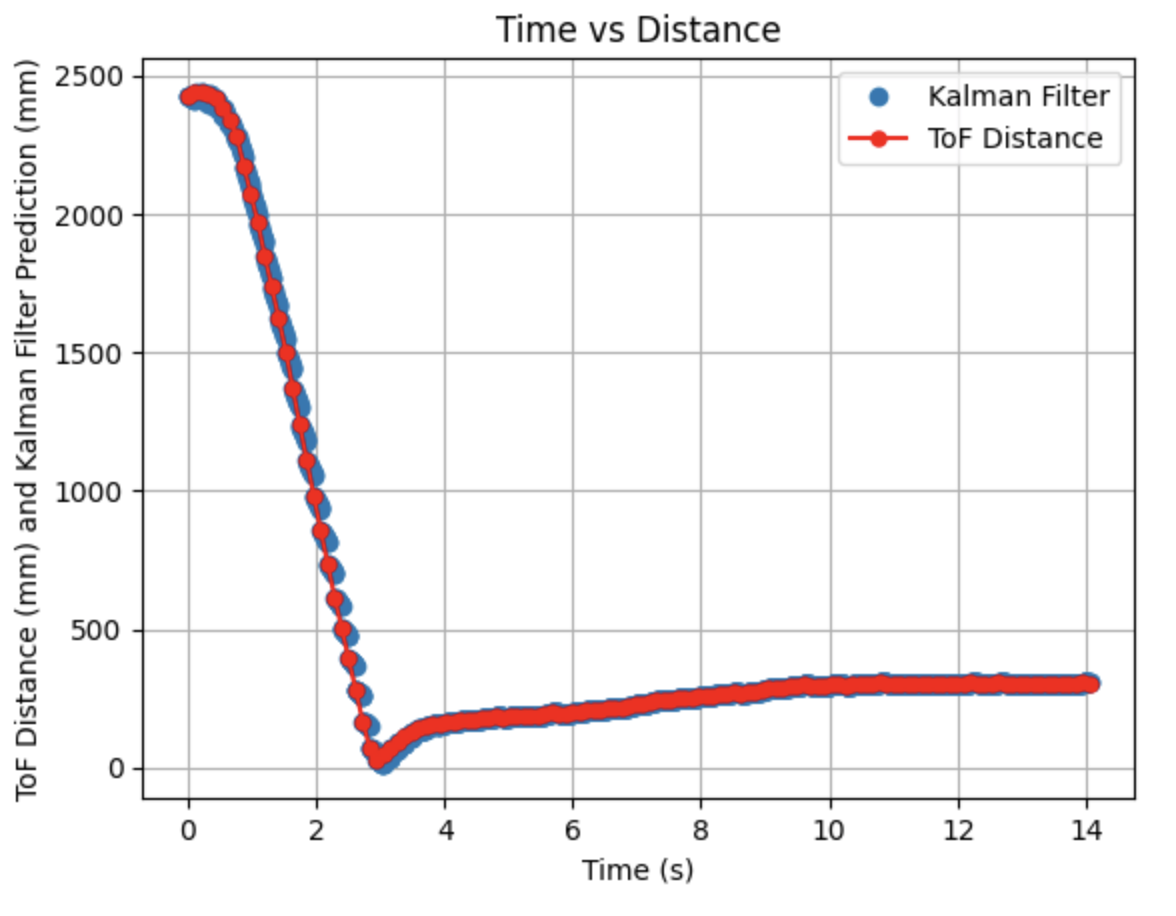
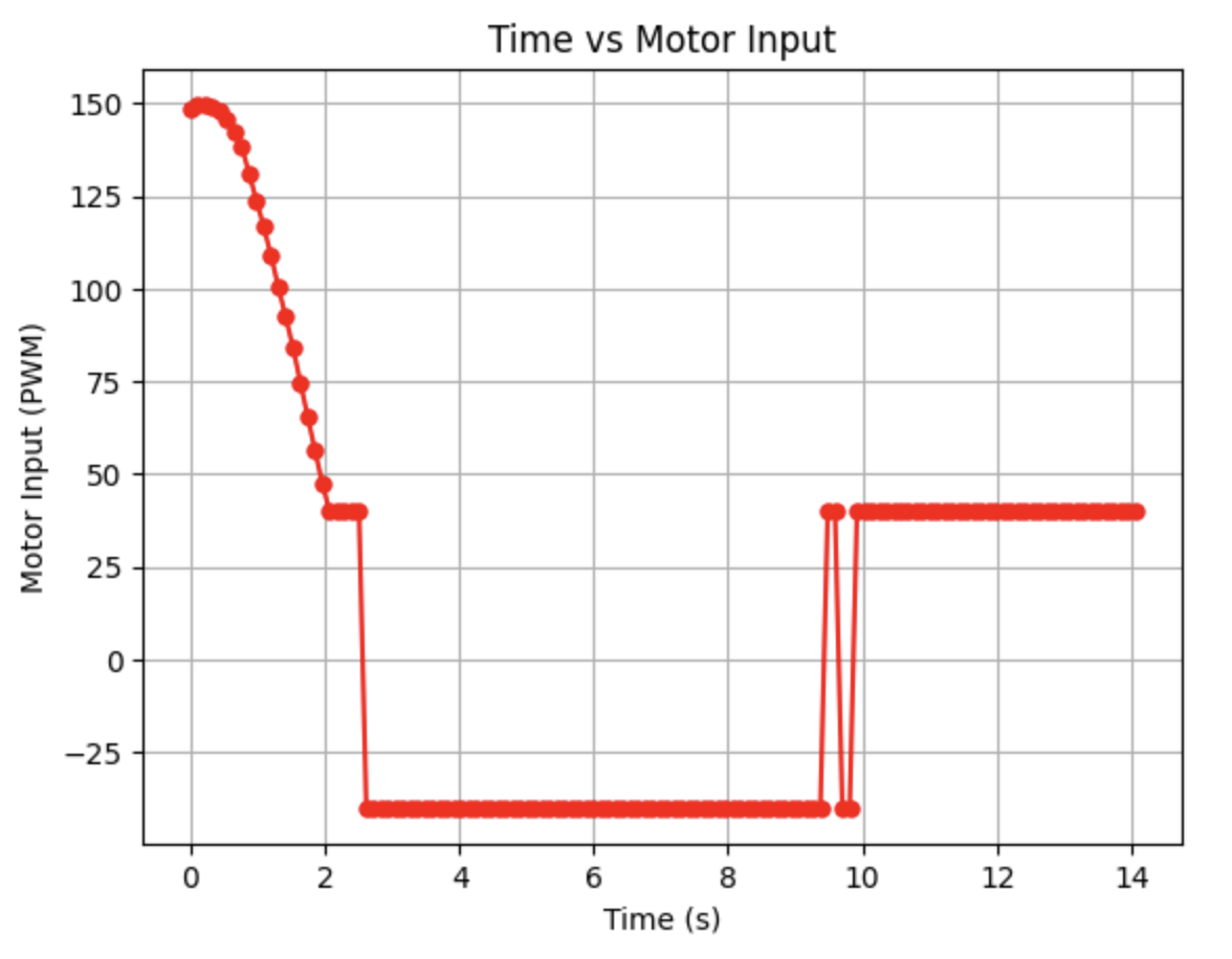
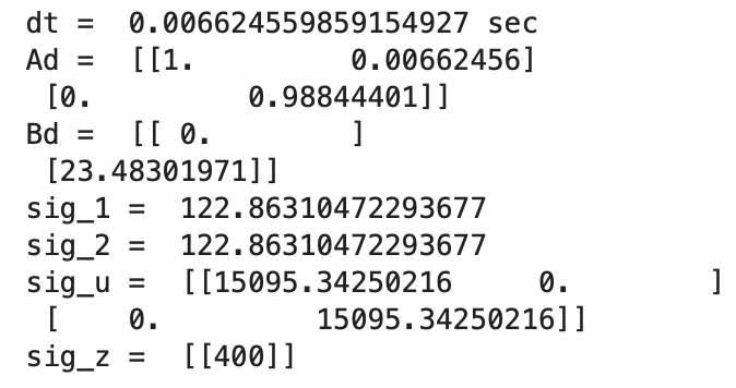
Initially running the Kalman Filter using the previously described code results in the above graphs. The calculated Delta_T for the PID controller is 0.0066 seconds, a frequency of 151.52Hz. The Kalman Filter is running at a faster frequency than the ToF sensors. The deadband for the motor controller input is 40. This deadband is consistent to the deadband used in Lab 5 for linear PID control. This was the fastest run of the robot with a maximum PWM value of 150. Sigma_1 and Sigma_2 are 122.86 and Sigma_3 is 20. Overall, the model works fairly well, but at around 2 seconds the predictions no longer extend to the next data point compared to the earlier predictions. In the next step I modify the parameters to adjust the prediction values.
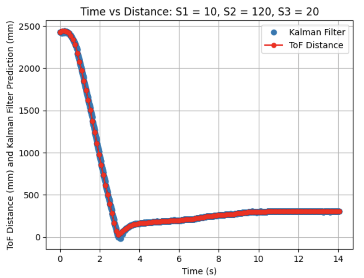
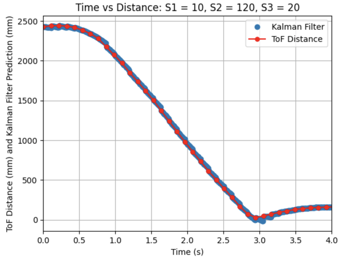
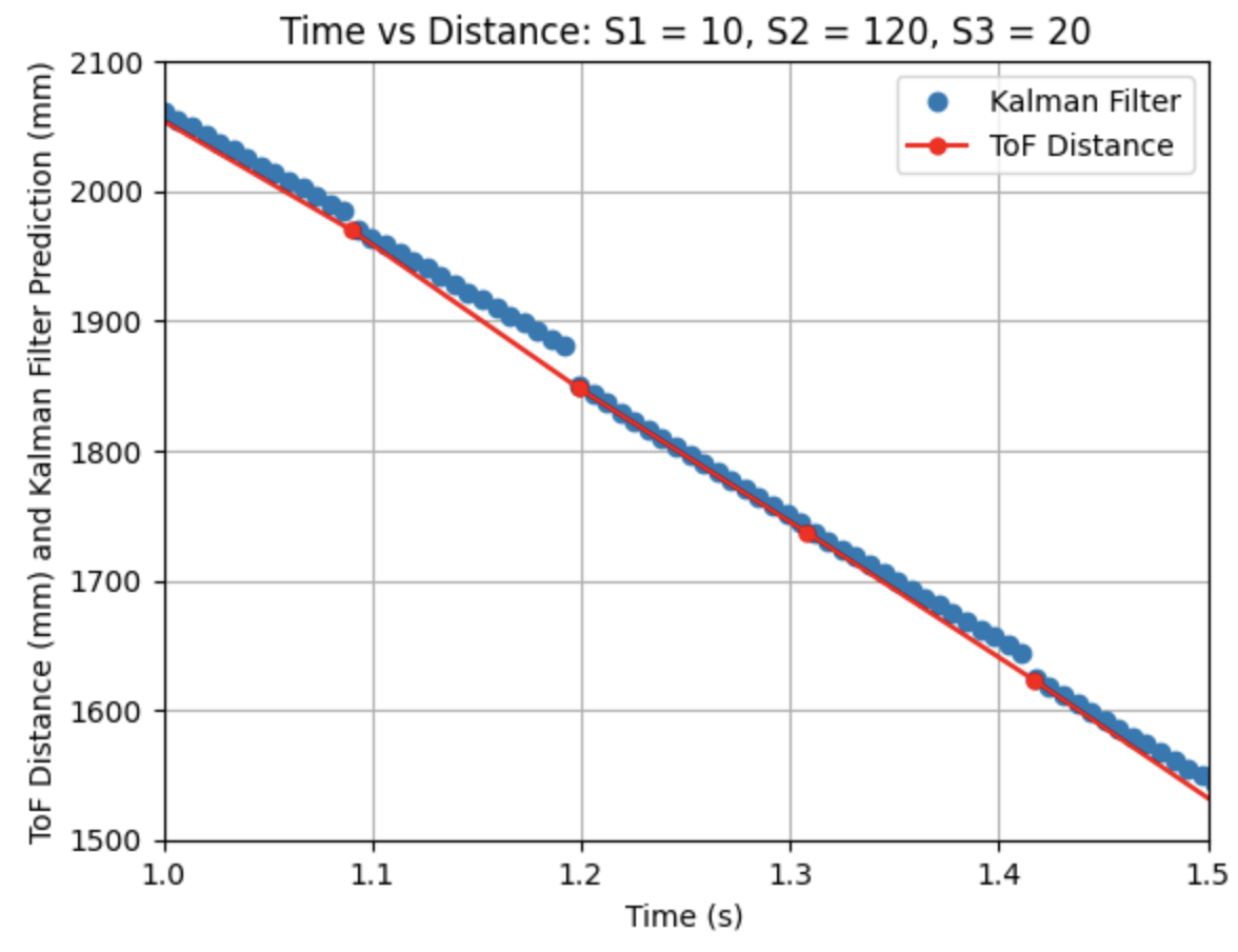
I adjusted the parameters for Sigma_1. Decreasing Sigma_1 (model uncertainty for location) indicates that the model is more accurate than what was initially predicted from the calculation for Sigma_1. Sigma_2 was set to 120, which is close to the initial calculated value found previously and Sigma_3 remains at 20. All other parameters (d, m, and Delta_T) were kept the same as the previous step. As can be seen from the graphs the Kalman Filter more closely follows the trend of the distance measurements.
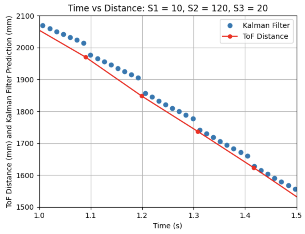
In the above graph I kept all previously found parameters the same but changed the value of the increment "i" in the while loop. The line changed from "i = i + Delta_T" to "i = i + 2*Delta_T". This change results in less Kalman Filter predictions to be plotted. I initially did this to better see the individually plotted prediction points, but then realized that changing how often the while loop runs the prediction step of the Kalman Filter results in the predictions to be slightly off from the ToF distance measurements and the previously plotted prediction values.
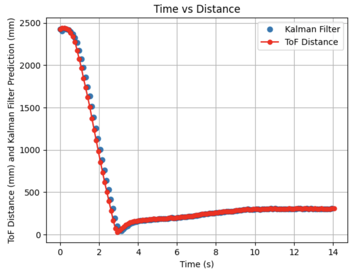
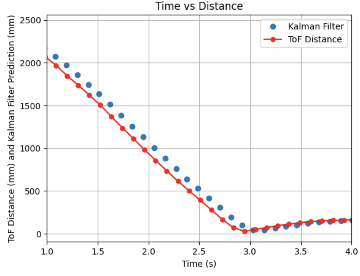
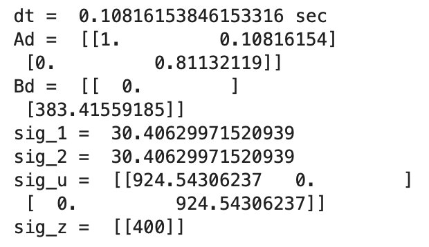
The above graphs show the Kalman Filter plotted without the prediction steps, only the updated values. The calculated Delta_T for the ToF sensor readings is 0.1082 seconds, a frequency of 9.24Hz. The Kalman Filter is running at the same frequency as the ToF sensors. Sigma_1 and Sigma_2 are 30.41 and Sigma_3 is 20. The Kalman Filter follows the general trend of the ToF readings, but is slightly off from the plotted line for the ToF distances. I tried modifying the parameters as I did in the previous step, but there was no significant change in the Kalman Filter updates.
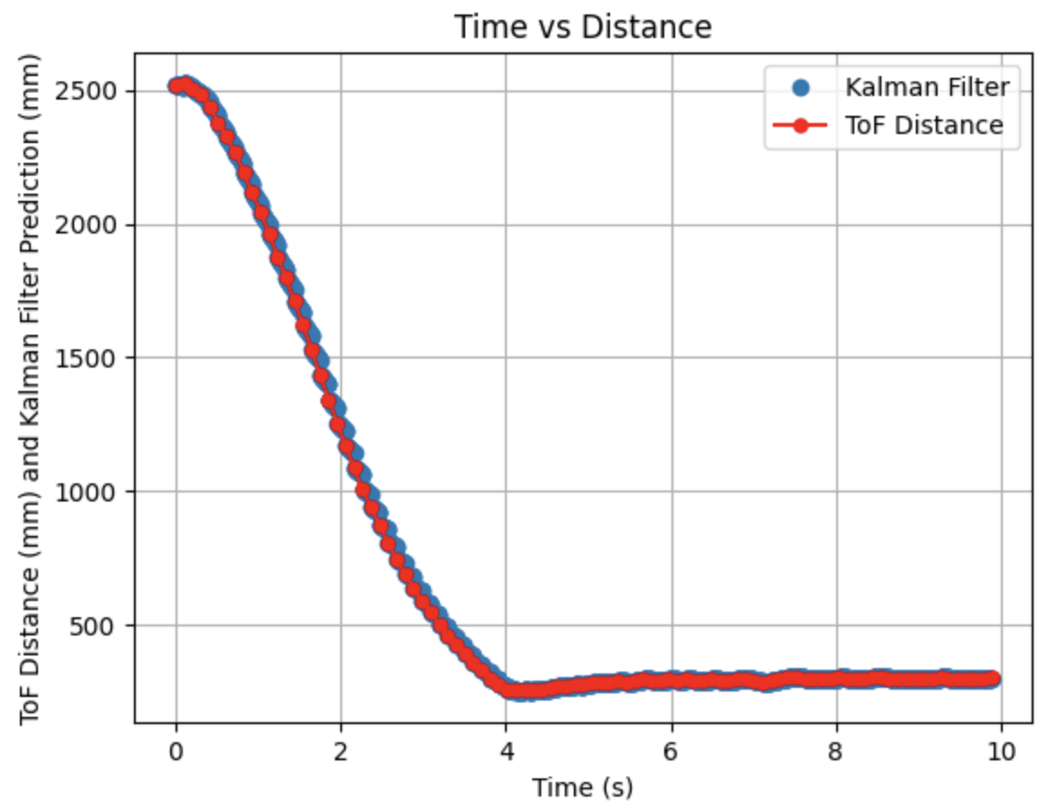
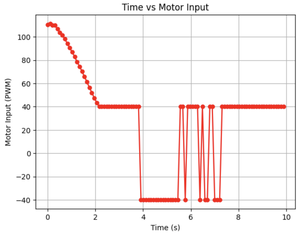
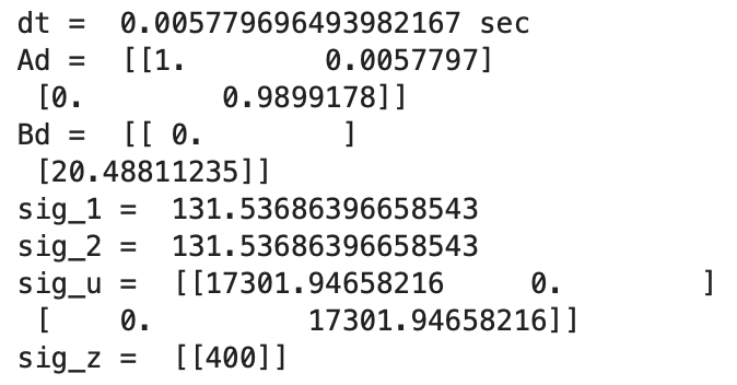
Initially running the Kalman Filter results in the above graphs. The calculated Delta_T for the PID controller is 0.0058 seconds, a frequency of 172.41Hz. The Kalman Filter is running at a faster frequency than the ToF sensors. The maximum PWM value is 115. Sigma_1 and Sigma_2 are 131.54 and Sigma_3 is 20. Overall, the model works well, but the predictions could be more inline with the ToF distances. In the next step I modify the parameters to adjust the prediction values.
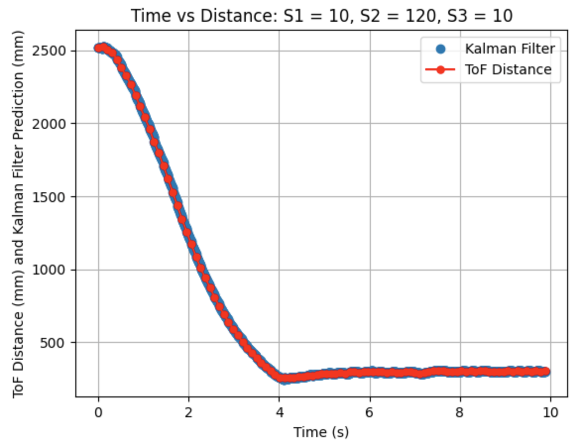
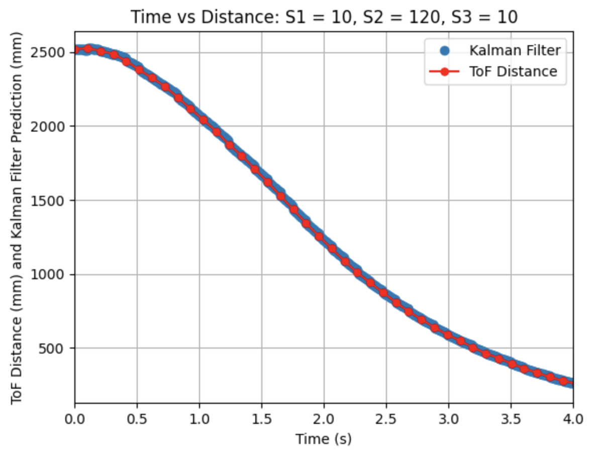
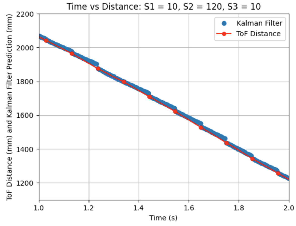
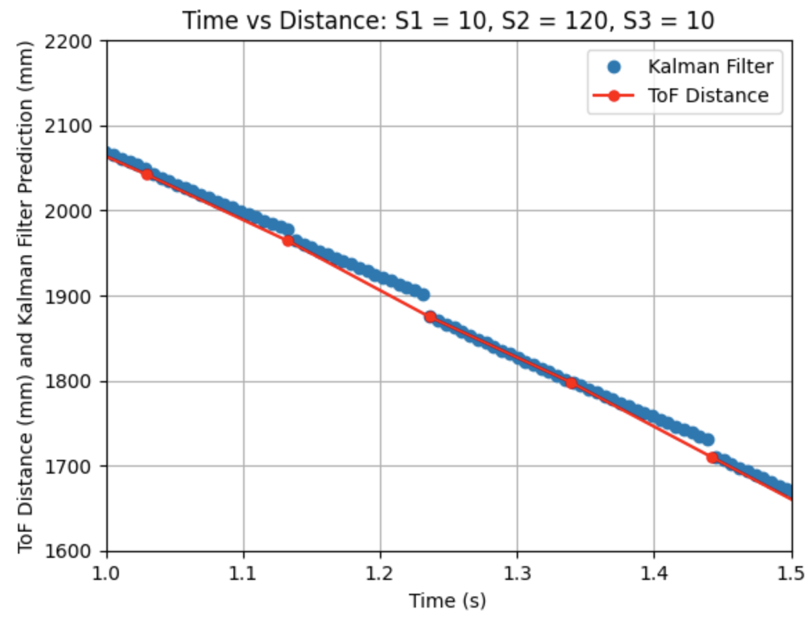
I adjusted the parameters for Sigma_1, Sigma_2, and Sigma_3. Decreasing Sigma_1 to 10 (model uncertainty for location) and Sigma_2 to 120 (model uncertainty for velocity) indicates that the model is more accurate than what was initially predicted. Sigma_3 (sensor uncertainty) was changed to 10 as the sensor readings were reliable. All other parameters (d, m, and Delta_T) were kept the same as the previous step. As can be seen from the graphs the Kalman Filter more closely follows the trend of the distance measurements.
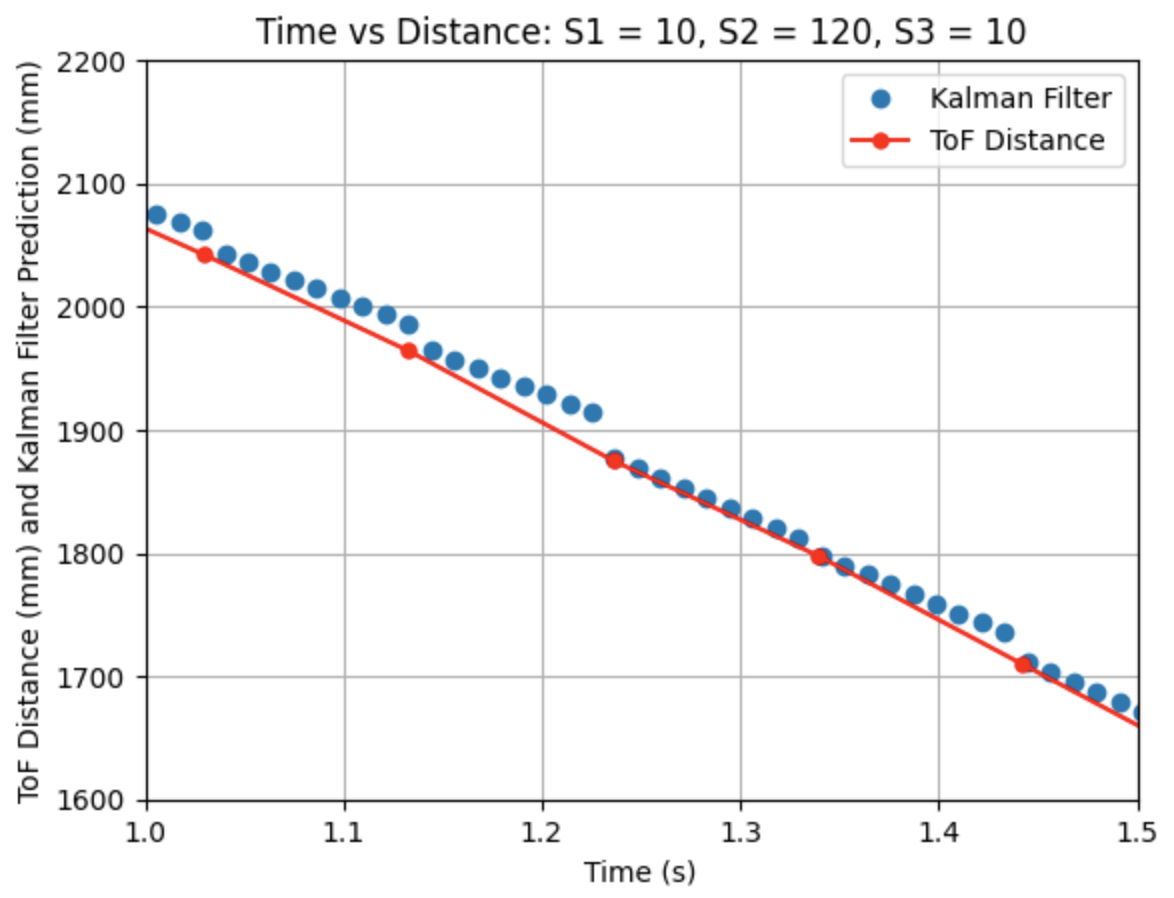
In the above graph I kept all previously found parameters the same but changed the value of the increment "i" in the while loop in the same manner as I did for Graph 1. The line changed from "i = i + Delta_T" to "i = i + 2*Delta_T". This change results in less Kalman Filter predictions to be plotted and the same offset behaviour as seen in Graph 1.
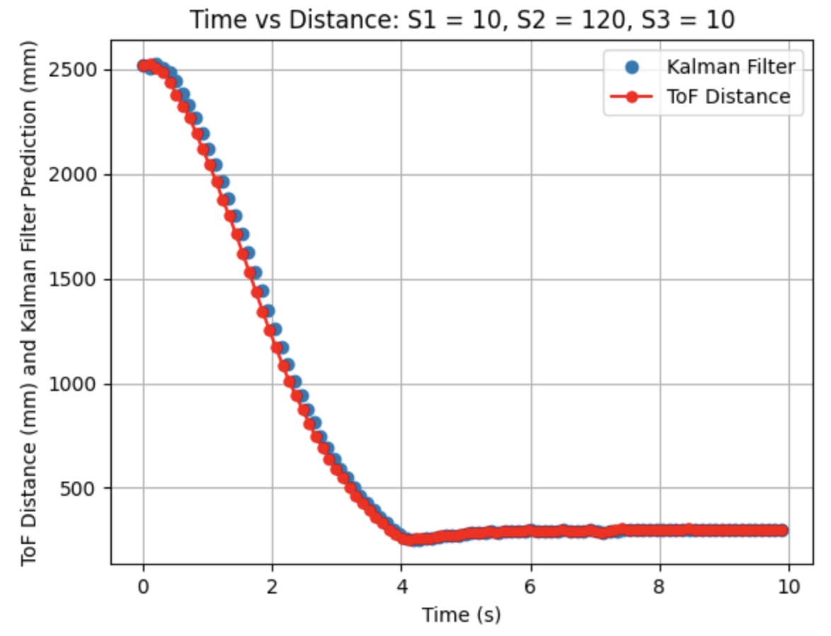
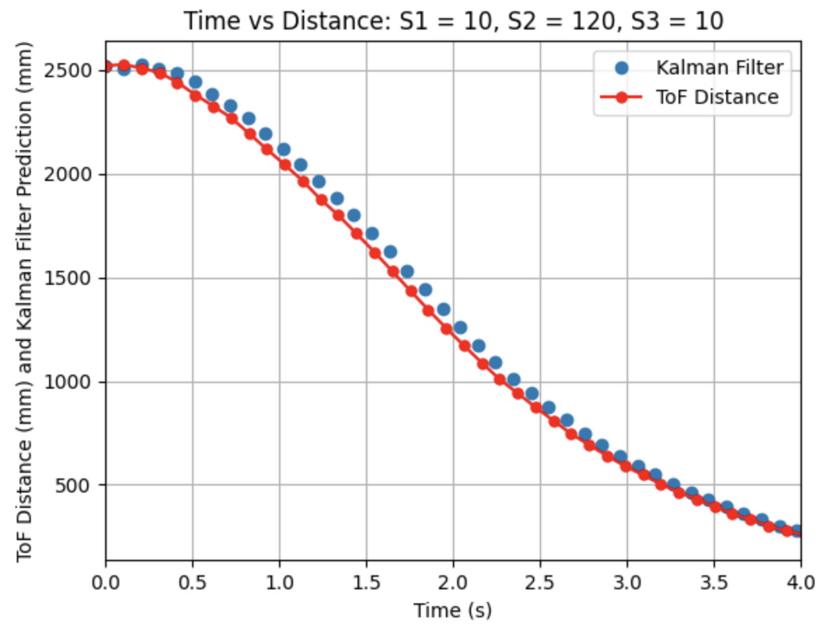

The above graphs show the Kalman Filter plotted without the prediction steps, only the updated values. The calculated Delta_T for the ToF sensor readings is 0.1019 seconds, a frequency of 9.81Hz. The Kalman Filter is running at the same frequency as the ToF sensors. Besides Delta_T, all other parameters were kept the same as in the previous step. The Kalman Filter follows the general trend of the ToF readings, but is slightly off from the plotted line for the ToF distances, although the plotted line is still closer to the ToF readings compared to Graph 1.
Prior to collecting the data to create the previous graphs, I tested the robot multiple times and collected distance readings. The distance readings were not as smooth as I would have expected and the robot moved slowly. I realized that my distance sensor was set to short mode, rather than long mode. The below data was collected before changing the sensor mode. I decided to run this data through the Kalman Filter for fun, to see how well the model would respond to non-ideal data.
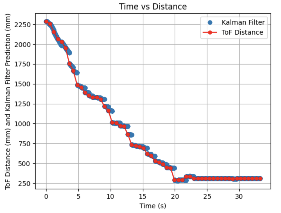
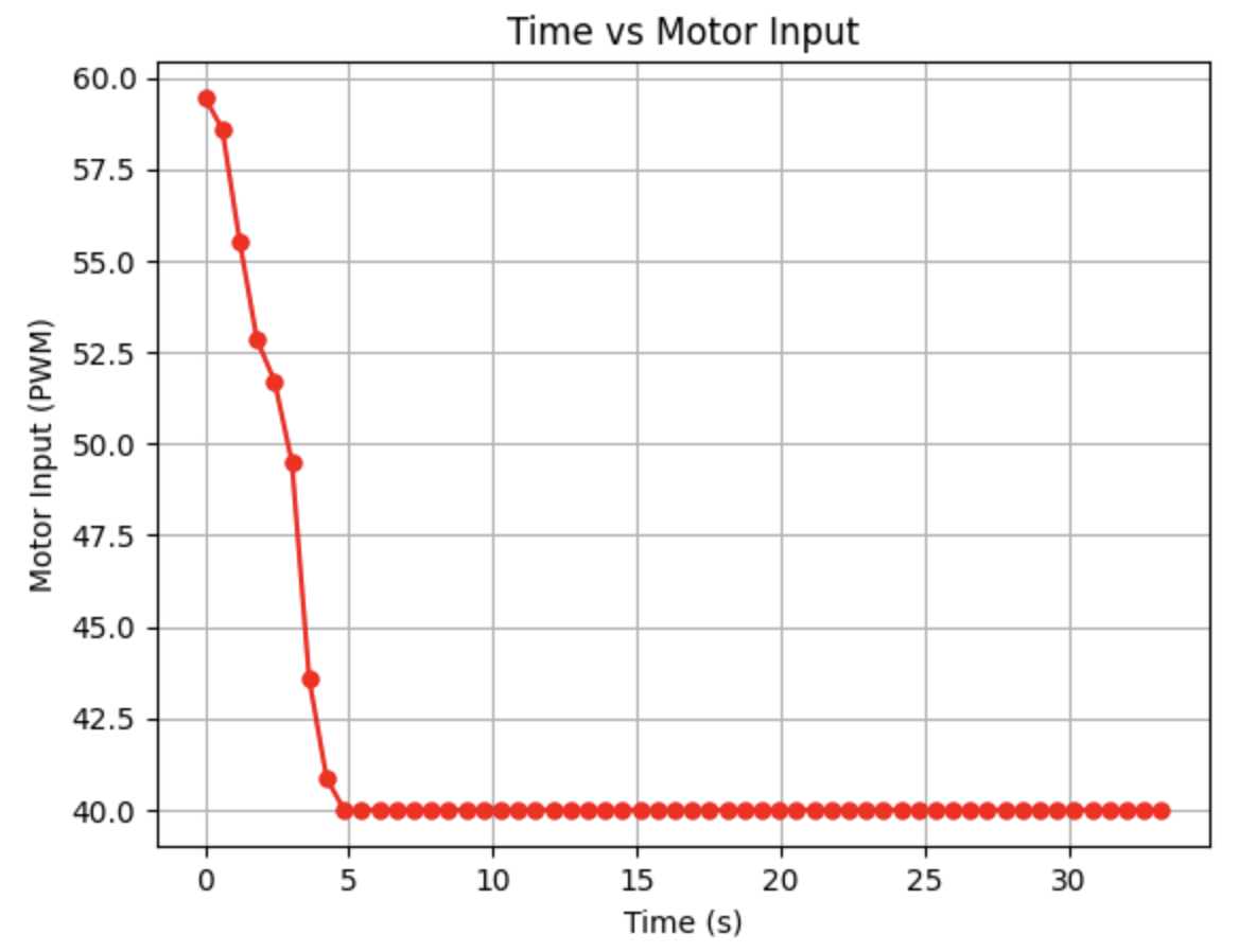

Initially, the Kalman Filter follows the ToF distance measurements, but later the predictions become more horizontal rather than continuing along the same slope as the distance sensor readings. I tried to address this issue in the next step.
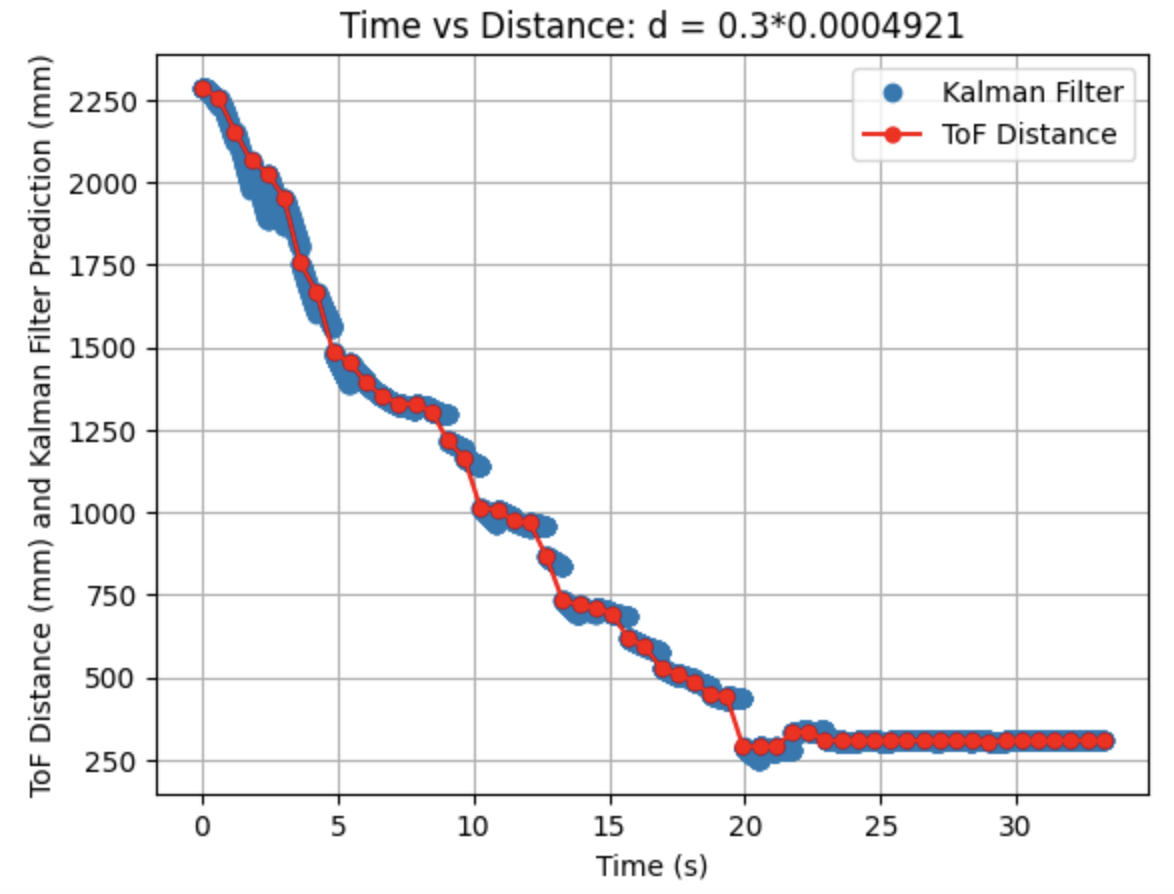
I adjusted the parameters and determined that decreasing the drag (d) constant resulted in a more downward trend of the calculated predictions. This trend was most significant towards the beginning of the graph.
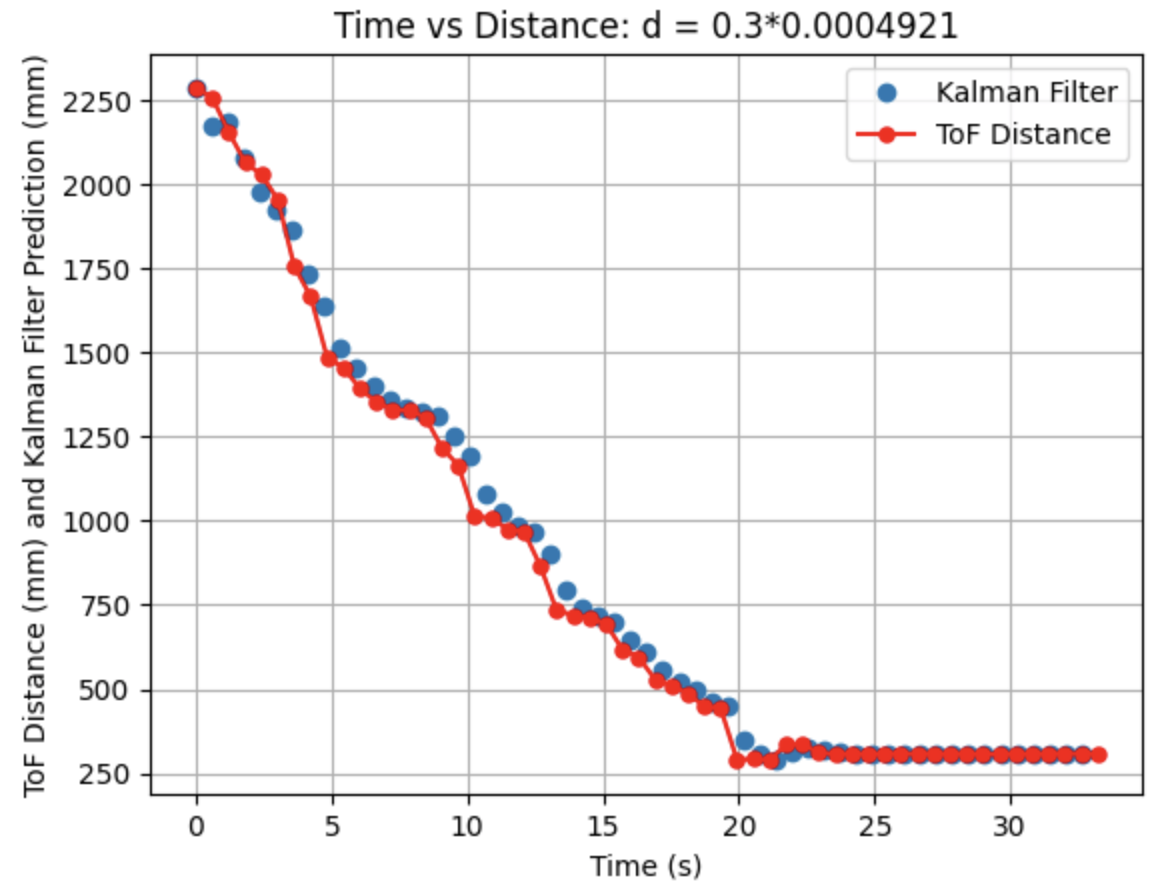
Above is the Kalman Filter plotted without the prediction steps.
I will include implementing the Kalman Filter on the robot for extra credit in the next lab report for Lab 8: Stunts.
Thank you!
Thank you to all of the TAs that answered my questions. I referenced the past lab reports of Liam Kain, Rafael Gottlieb, Larry Lu, Julian Prieto, and Ignacio Romo.
The objective of the lab to to gain experience working with PID controllers for orientation. I am a 5000 level student and I choose to work on a PID controller. Labs 5-8 detail PID, sensor fusion, and stunts. This lab is focused on using a PID controller for orientation control of the robot. The IMU will be used to control the yaw of the robot.
I replaced one of my motor drivers that was overheating due to some solder touching between pins after I had to reconnect a loose wire. The new motor driver and connections solved the issue.
I considered using tape around the wheels to reduce friction with the ground, but decided that I did not want to change the surface of the wheels. During the lab I found the lower limit PWM value for turning and implemented the found value as a lower limit for the motor control functions. The surface of the wheels is consistent with all past labs as I have previously found lower limit PWM values for forwards/backwards motion using both wheels and one wheel, starting from stationary and moving at a constant speed before lowering the PWM. All of my found lower limit PWM values are for the same wheel surface.
The lab materials include:
For this lab a PID controller will be used for orientation control of the robot. The below equation from the course Lecture 7 is used to compute the value for the PID controller:

This equation uses the error e(t) (difference between the final desired value and the current value) in proportional, integral, and derivative control to calculate the new PID input value u(t). For this lab the error is the difference between the desired angle (yaw) and the robots current angle (yaw). The calculated PID input value is related to the robots angular speed. Proportional control multiplies a constant Kp by the error. Integral control multiplies a constant Ki by by the integral of the error over time. Derivative control multiplies a constant Kd by the rate of change of the error.
For Lab 6 data was sent over Bluetooth in the same manner as the previous Lab 5.
Two Arduino IDE cases were initallized. The case ORIENTATION_CASE starts and stops the PID controller and the case SEND_ORIENTATION_DATA sends the collected PID data to Jupyter Notebook. The PID controller starts when a command from Jupyter Notebook is run. The command inputs include a start(1)/stop(0) value; the desired setAngle value to determine the desired angle; and the Kp, Ki, and Kd constant values. In Jupyter Notebook a notification handler similar to the notification handler from Lab 1 is used to create the data array. The PID controller stops when the first input value is set to zero.
I also determined what data I wanted to store and send to Jupyter Notebook. I stored the time, yaw, error, proportional value, integral value, derivative value, PID value, right motor input, left motor input, and the setAngle value.
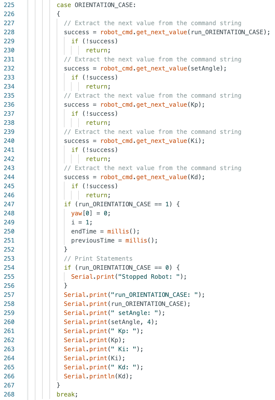
Below is the Jupyter Notebook Command and corresponding Arduino case to start/stop the PID controller. The run_ORIENTATION_CASE, setAngle, Kp, Ki, and Kd values sent from Jupyter Notebook are printed in the Arduino serial monitor each time a command is sent. These values were initalized as global variables and will be used in the PID controller that is written in the main void loop(). If a command to stop the robot is sent from Jupyter Notebook "Stopped Robot: " will also be printed in the Arduino serial monitor.

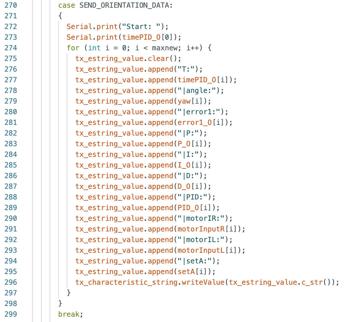
Below is the Jupyter Notebook Command and corresponding Arduino case to send the collected data. When data is sent the first time value is printed to the Arduino serial monitor to confirm that data was sent to Jupyter Notebook correctly. The time value is compared to the first time value in Jupyter Notebook.

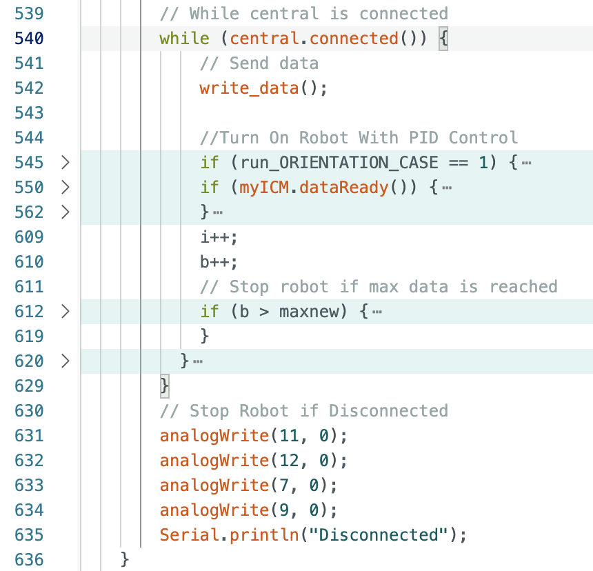
The same hard stop used in Lab 5 is used in Lab 6 as well to stop the robot if Bluetooth connection is lost.
The above link has the full final version of the code used during the lab. I attached the link for my own reference in the future. The below steps show how and why I wrote each piece of the code.
The gyroscope reading was integrated using the following lines of code:

These lines of code are within the larger while loop and each time the while loop runs the gyroscope updates the sensor readings. Yaw is then found using the previous yaw reading, the gyroscope reading, and the calculated difference in time.
A potential problem with digital integration includes not having available data to properly integrate. The if statement to read IMU data only runs when data is ready. If data is not ready then the PID controller will not be using the most current angle available. If there is no ready gyroscope data over time this might cause an issue. I observed the angle readings throughout the lab procedure and did not notice any significant gaps in data for the yaw calculations. Another potential problem is gyroscope drift. If the IMU is continuously used the gyroscope readings will drift away from the actual angle of the robots location. To address this issue, I set the initial yaw reading to zero every time I started using the PID controller.
Potential IMU sensor bias includes the placement of the IMU on the robot. If one of the IMU axis is not aligned with the center of the robot or if the IMU is not centered on the middle axis, then the calculated angle from the gyroscope sensor reading may not align with the physical location of the robot.
I also checked to see if there was any numerical initial bias in the yaw calculations from the gyroscope by printing yaw readings to the Serial Monitor. I did not observe any bias when starting the PID controller.
The gyroscope sensor has four selections for rotational velocity. The selections are (+/-)250, (+/-)500, (+/-)1000, and (+/-)2000 degrees per second. This information is from this datasheet. Of the four potential configurations the settings of (+/-)500, (+/-)1000, and (+/-)2000 degrees per second will work for the purposes of this lab. The maximum angle that could potentially be used for robot motion control is 360 degrees, while smaller angles of 180 degress or less are preferred. The gyroscope configuration of (+/-)500 will be used to ensure that all potential gyroscope sensor data is collected.
Other limitations of the sensor include being compatible with 3.3V or 5V, having 9 degrees of freedom, and the accelerometer has four configurations including (+/-)2g, (+/-)4g, (+/-)8g, and (+/-)16g. The accelerometer will not be used for this lab.
For the orientation control task the robot uses a PID controller and the calculated yaw angle from the gyroscope readings to move towards and maintain the set angle. The implemented PID controller works for various angles and on different floor surfaces.
The calculated yaw error from the gyroscope sensor can be at most 360 degrees. To determine the sampling time of the gyroscope readings I found the time between each new IMU measurement by temporarily adding a Serial.print(dt_G); line to the if statement inside of the while loop. The sampling period was found to be 0.01s, resulting in a sampling frequency of (1/0.01s) = 100Hz for IMU measurements.
To find how fast the PID control loop is running I temporarily adding a Serial.print(dt_O); line inside of the while loop for the PID controller. The PID loop runs at around 0.01s (1/0.01s = 100Hz). The PID loop is running at around the same speed as the gyroscope sensor readings.
While I was initially testing the PID controller the lower limit PWM value was set to the same as the lower limit value of 40 from the previous lab. Using a lower limit of 40 resulted in the robot getting stuck and not fully turning. I created a new Arduino case and Jupyter Notebook command to find the lower limit PWM for turning. The code is below:

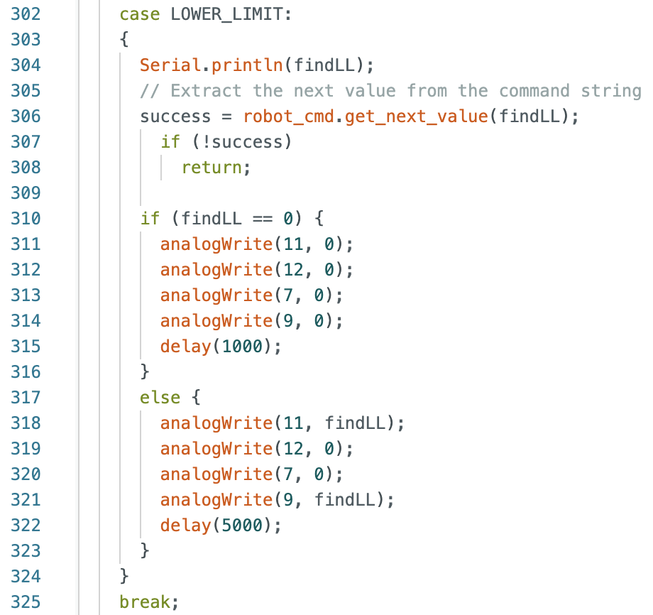
After testing various PWM values, I found that a lower limit value of 120 resulted in the robot turning. A video of the robot at a PWM value of 120 is below:
The Arduino code for PID control is below:
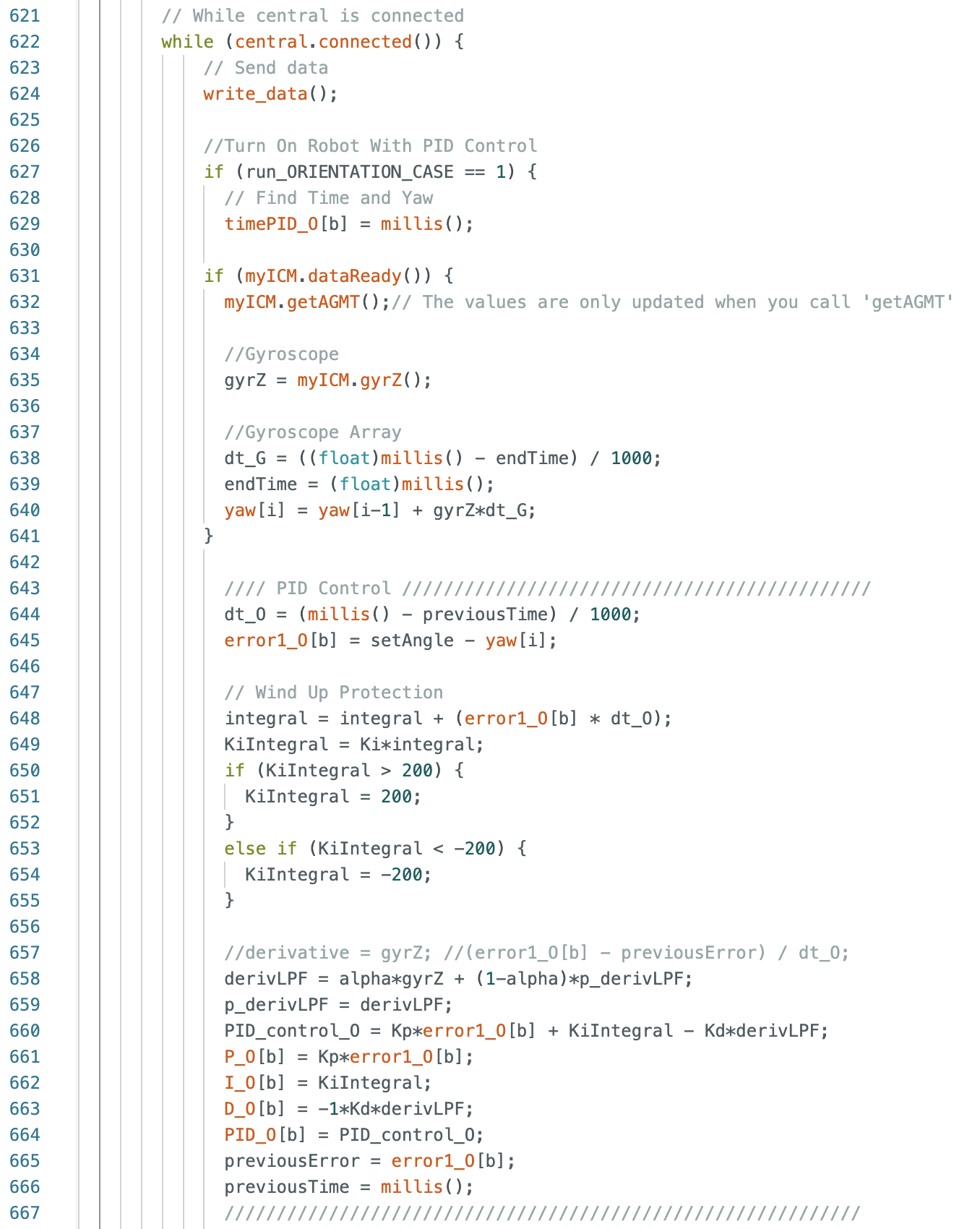
Within the while loop if run_ORIENTATION_CASE is equal to 1, then the PID controller will run. First the time is recorded and then data for the gyroscope is collected and yaw is found. The error is the desired angle minus the yaw angle. The proportional control component is the error multiplied by Kp (within line 660). The integral control component is the error integrated over time multiplied by Ki (lines 649 and 650). Wind up protection is used in lines 651-656. If the value of the integral term multiplied by the set Ki value is greater than 200 then there will be no further increase in the KiIntegral term used to find the value for the integral controller. Without wind up protection the integral term will continuously increase causing the robot to not stop when the final yaw angle is reached. The derivative control componenet is the rate of change of the error multiplied by Kd (lines 658 and 659). The derivative controller uses a low pass filter and the gyroscope reading (gyrZ) as an input to reduce derivative kick when changing the setpoint.
The PID controller works for both positive and negative angles. Inputs of positive angles turn the robot counter clockwise. Inputs of negative angles turn the robot clockwise.
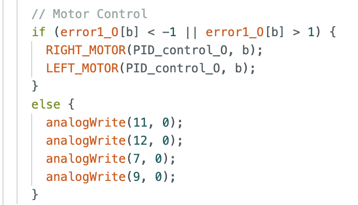
The robot is set to stop when the calculated error is less than 1 degree. All pins are then set to zero. If the error is not within the stopping range than the functions RIGHT_MOTOR and LEFT_MOTOR are called. The if statements and functions can be found below.
Stop when error is 1 degree or less or continue motion:
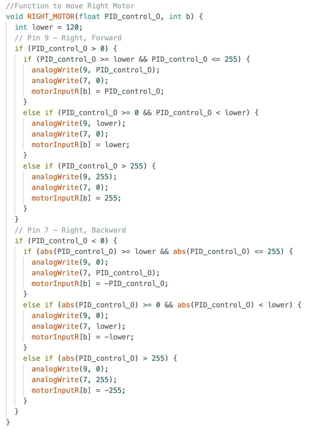
Right Motor:
Left Motor:
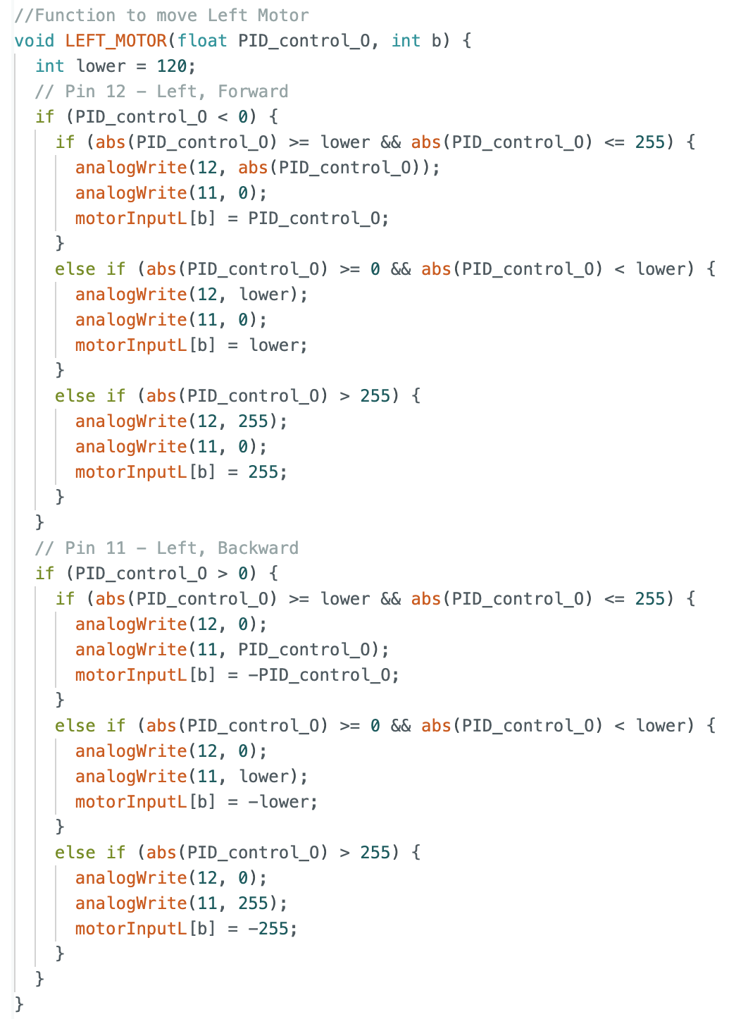
For PID values greater than or equal to 120 and less than or equal to 255, the PID value is used as the input PWM value for the motors. For values greater than 0 and less than 120 the input PWM value is set to be 120, because PWM values less than 120 result in no motion of the robot. For values greater than 255, the PWM value is set to 255 as that is the maximum possible value for the motors.
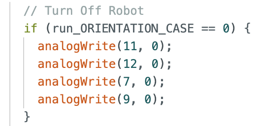
The two other ways to stop the robot are the same as in Lab 5. The first way is intentionally stopping the robot by sending a "0" value for run_ORIENTATION_CASE in Jupyter Notebook. Sending a "0" causes the following if statement in the while loop to set all pins to zero.
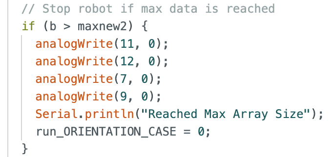
The second way that the robot stops is if the maximum value for the collected arrays is reached, causing all pins to be set to zero and stopping the robot. This is to ensure that each time the robot runs I know if the maximum array size is reached.
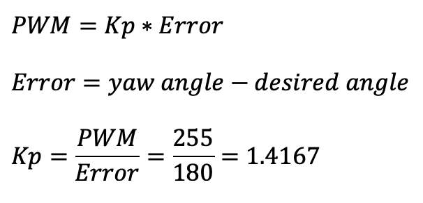
I started with testing the proportional controller. I worked on finding a value for Kp, while keeping Ki and Kd zero. I choose an angle of 180 degrees to start testing the proportional controller. I estimated the Kp constant to be 1.4167 when testing 180 degrees. The equations are found below:
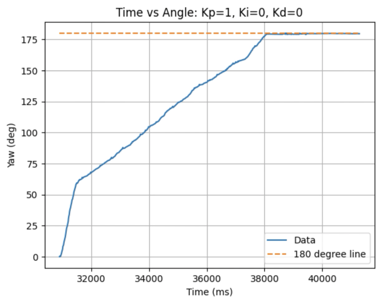
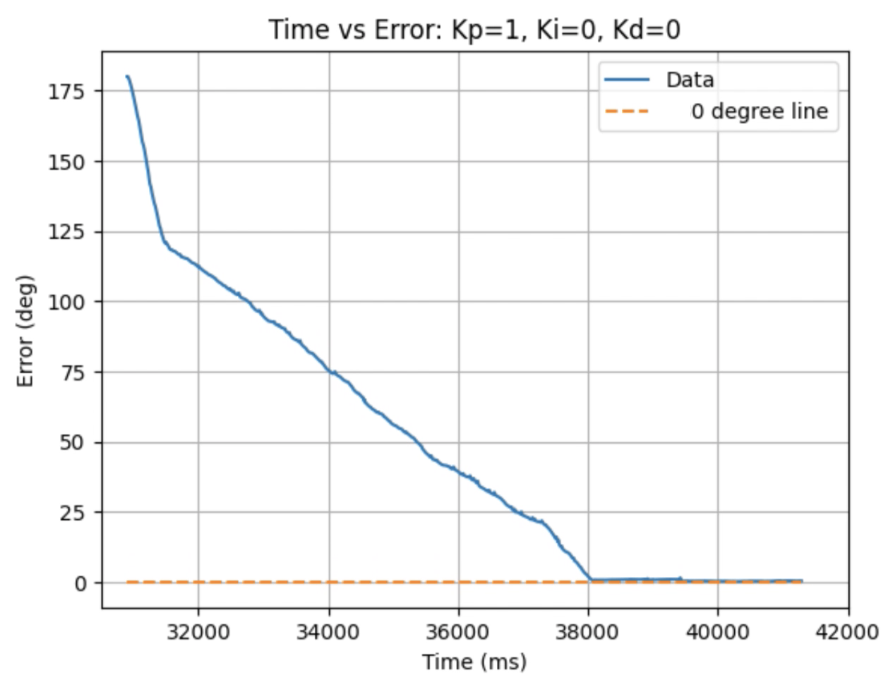
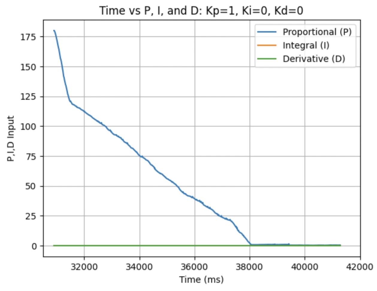
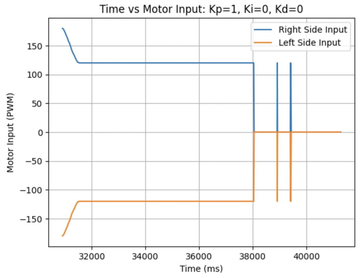
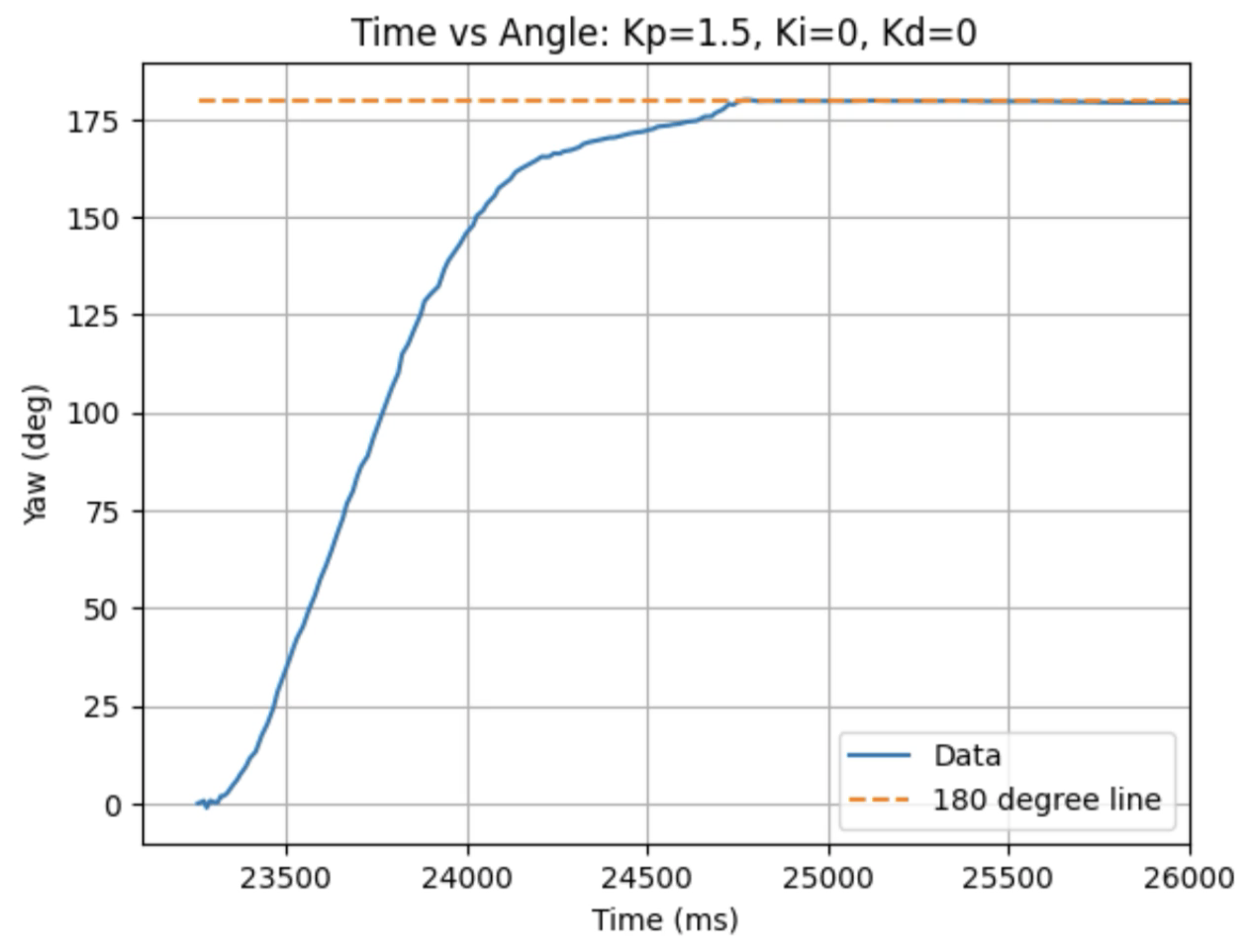
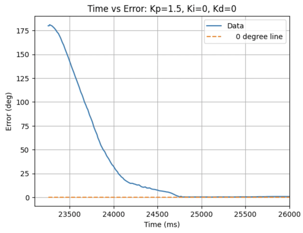
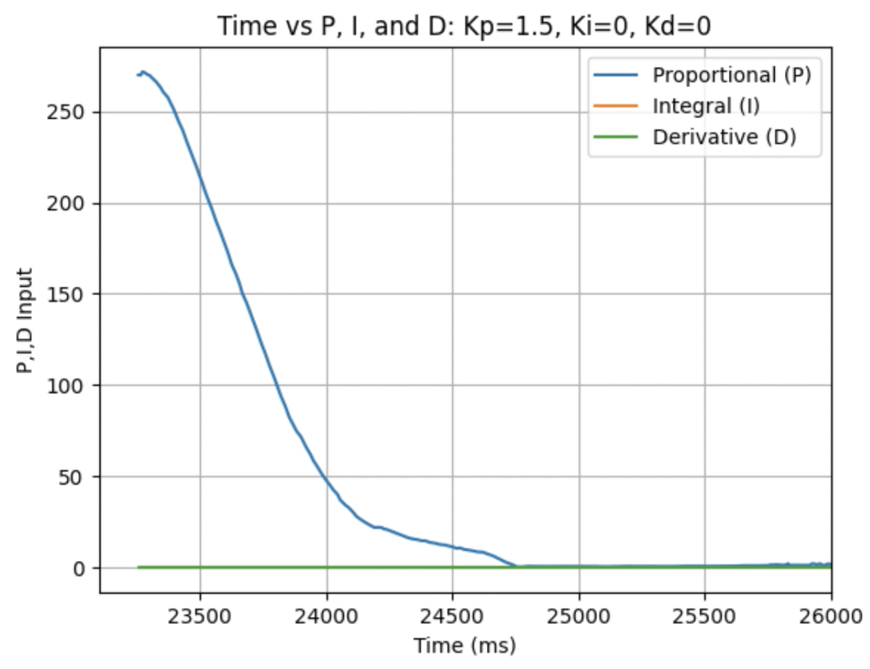
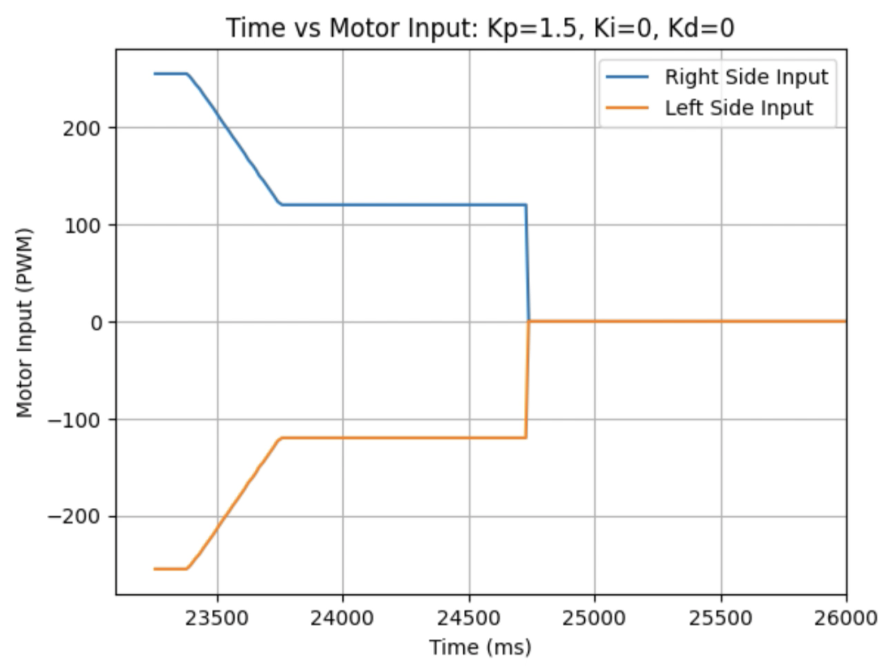
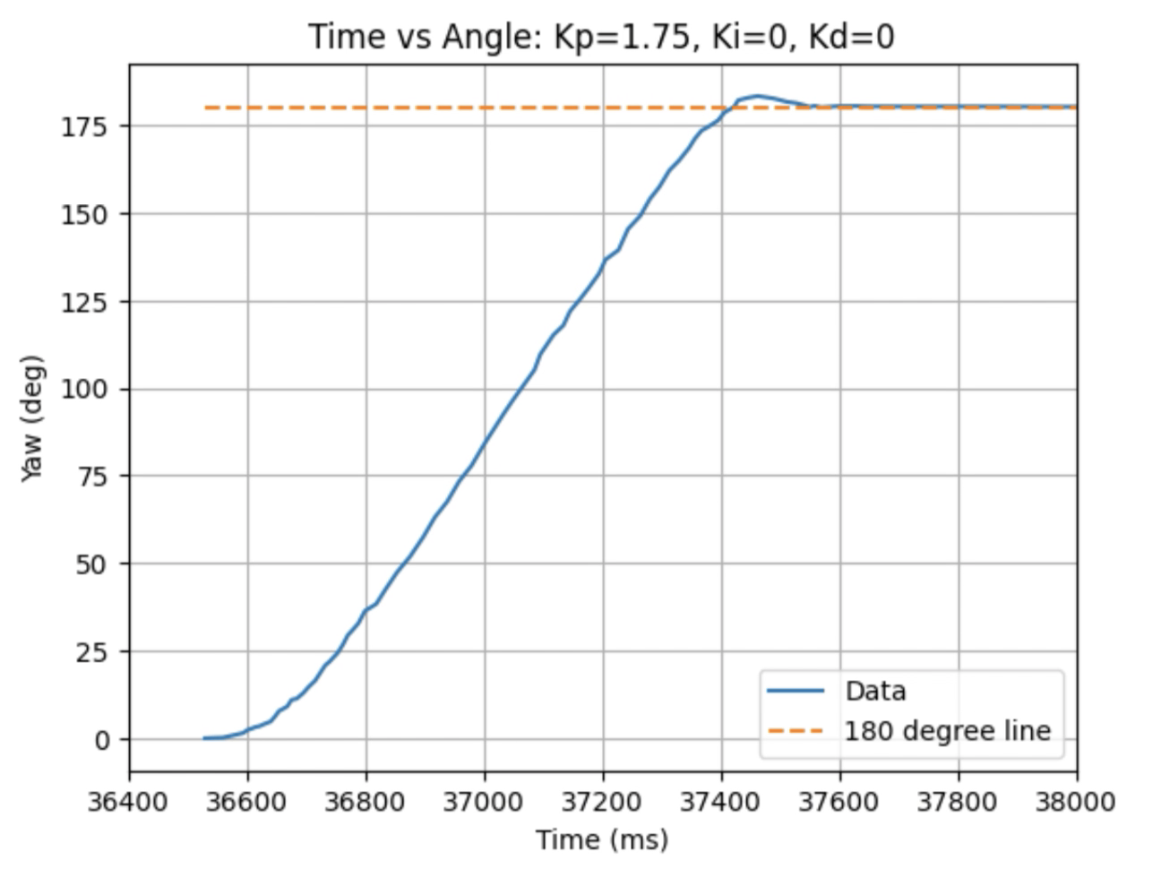
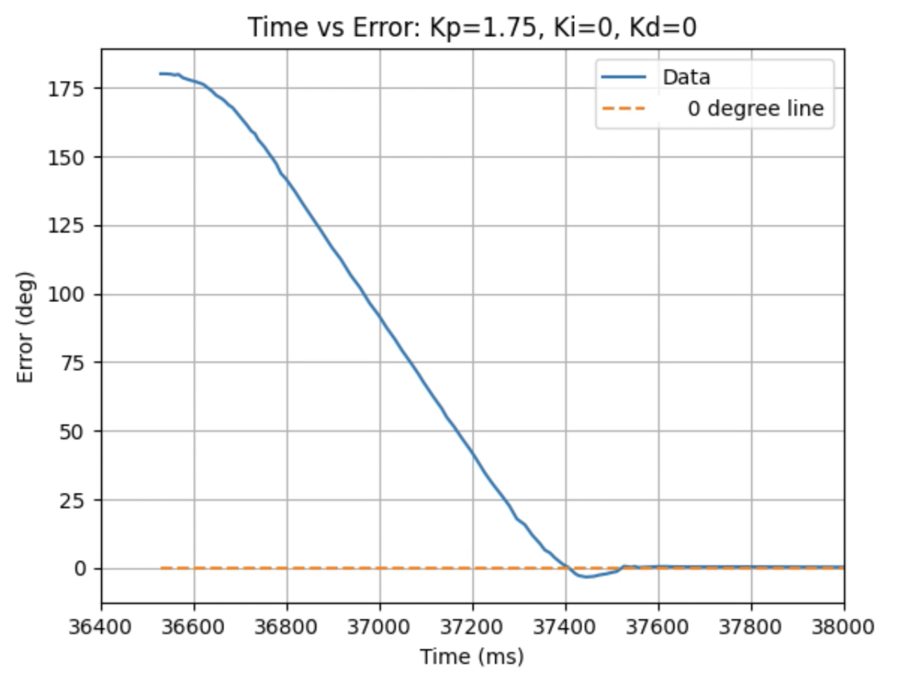
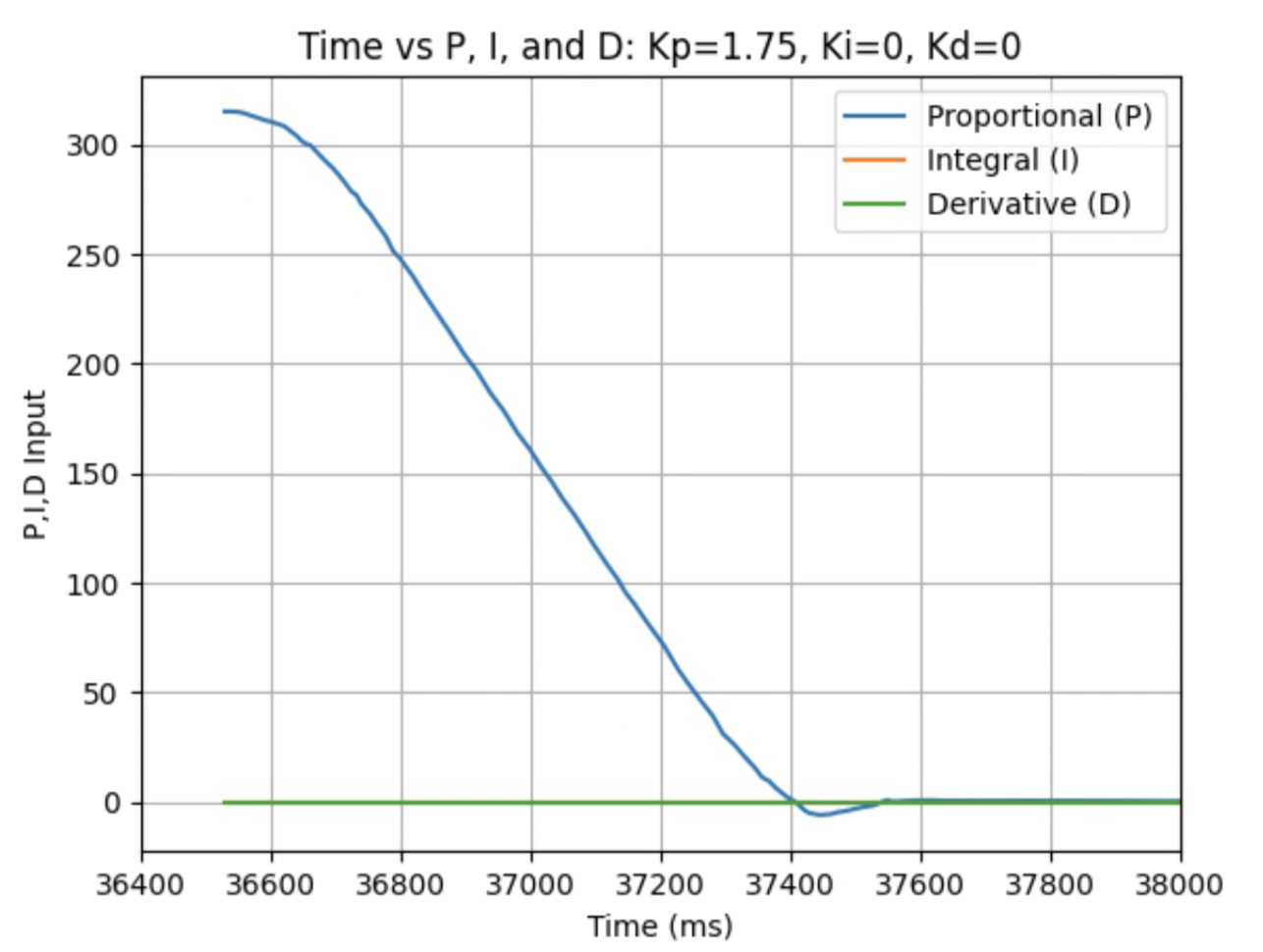
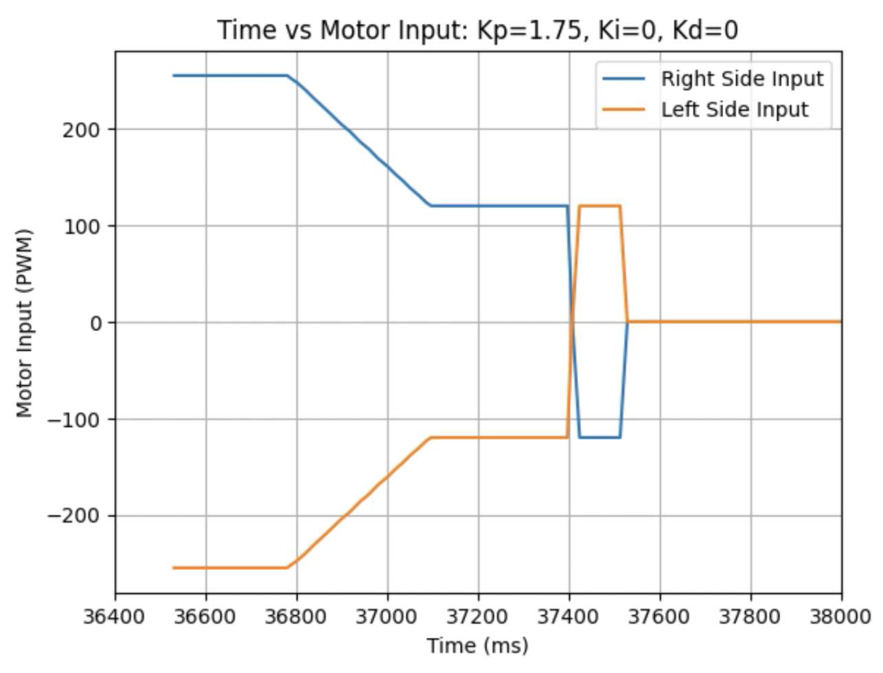
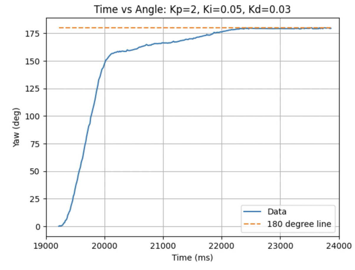
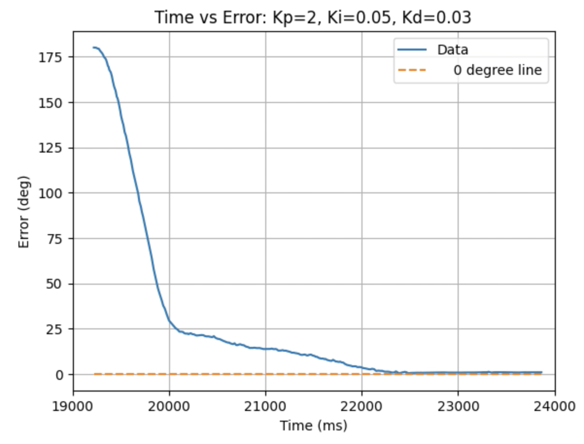
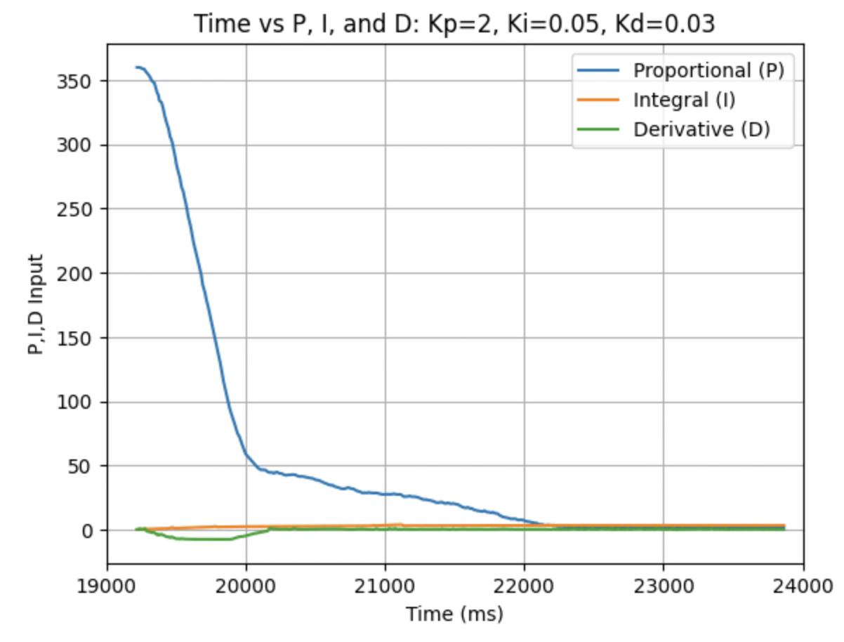
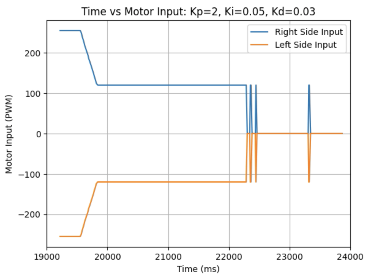
During physical testing I wanted the proportional control to slightly over shoot the desired angle. The over shoot will be addressed using derivative control and the speed will be addressed using integral control. A range of Kp values including 1, 1.5, 1.75, and 2 were tested as can be seen in the below graphs showing yaw, error, PID components, and motor input. I determined that the Kp value should be 2. The code for the proportional controller is below:
Graphs for Kp = 1:
Graphs for Kp = 1.5:
Graphs for Kp = 1.75:
Graphs for Kp = 2:
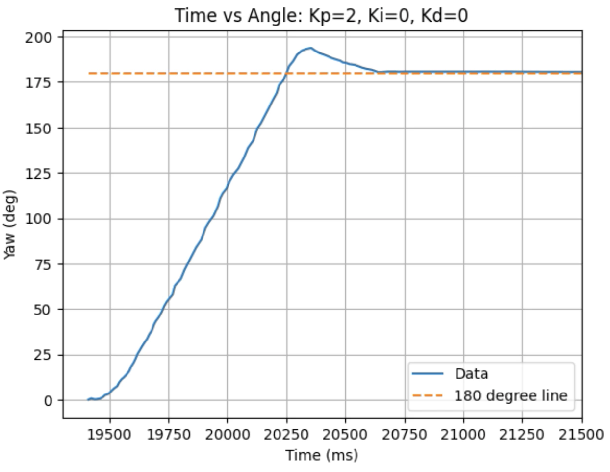
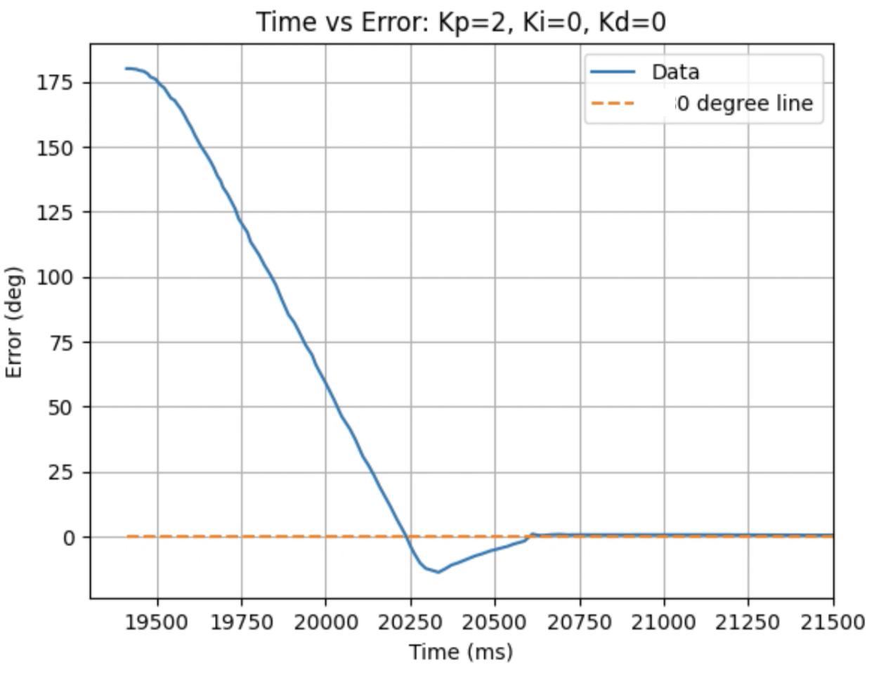
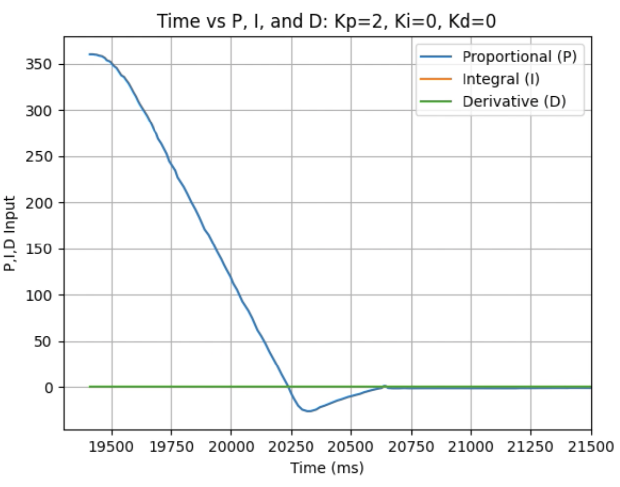
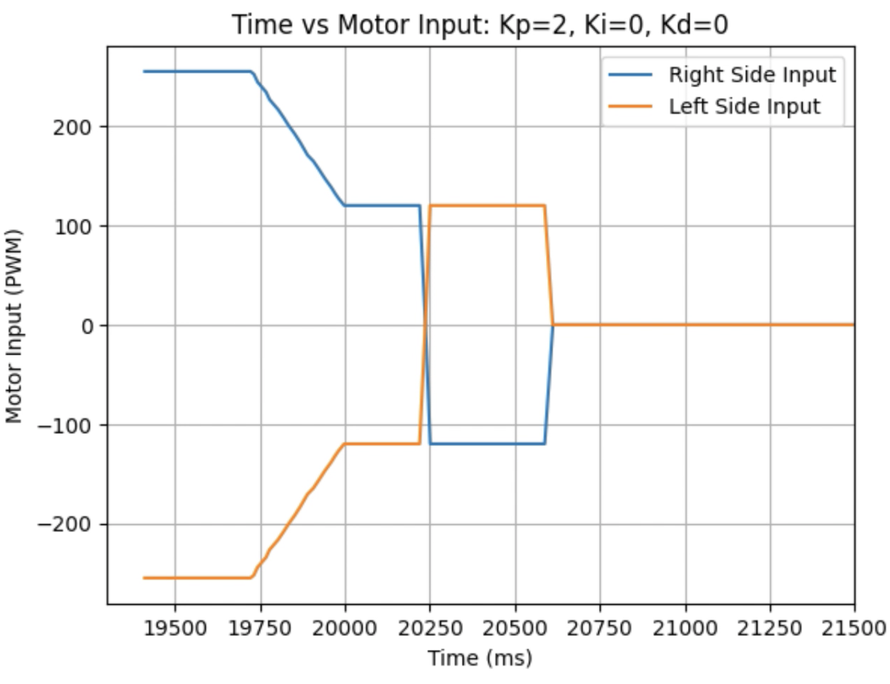
Trends that can be observed include, as the value for Kp increases the amount of time the robot takes to reach the desired angle decreases, but there is also more overshoot observed. As the value of Kp increases the motor input spends less time at the lower limit value of 120. For example, it is noticeably observed that for Kp = 1 the motor quickly reach the input value of 120 and remains at that value until the desired angle is reached. For Kp = 2 the motors start at the upper bound of 255 and then decrease to the lower limit of 120 before reaching 180 degrees. I choose a value of Kp = 2 to then move to testing the proportional and integral controllers together.
The next step involved using the proportional controller (with Kp = 2) and the integral controller to increase the speed of rotation and to achieve a small amount of oscillation at the desired angle. The integral controller is the constant Ki multiplied by integrated error over time. As time increases the integrated error increases, resulting in a greater contribution of the integral controller. To prevent the integral controller component from increasing continuously, wind up protection was implemented. If the value of Ki mulitplied by the time integrated error is greater than 200 or less then -200, then the KiIntegral is set to be 200 or -200 and does not further increase/decrease. The code for the proportional and integral controller is below.
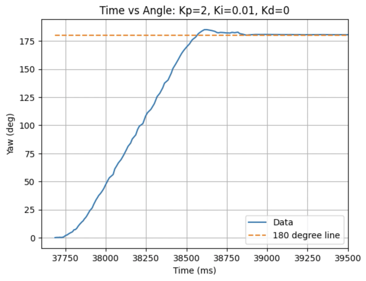
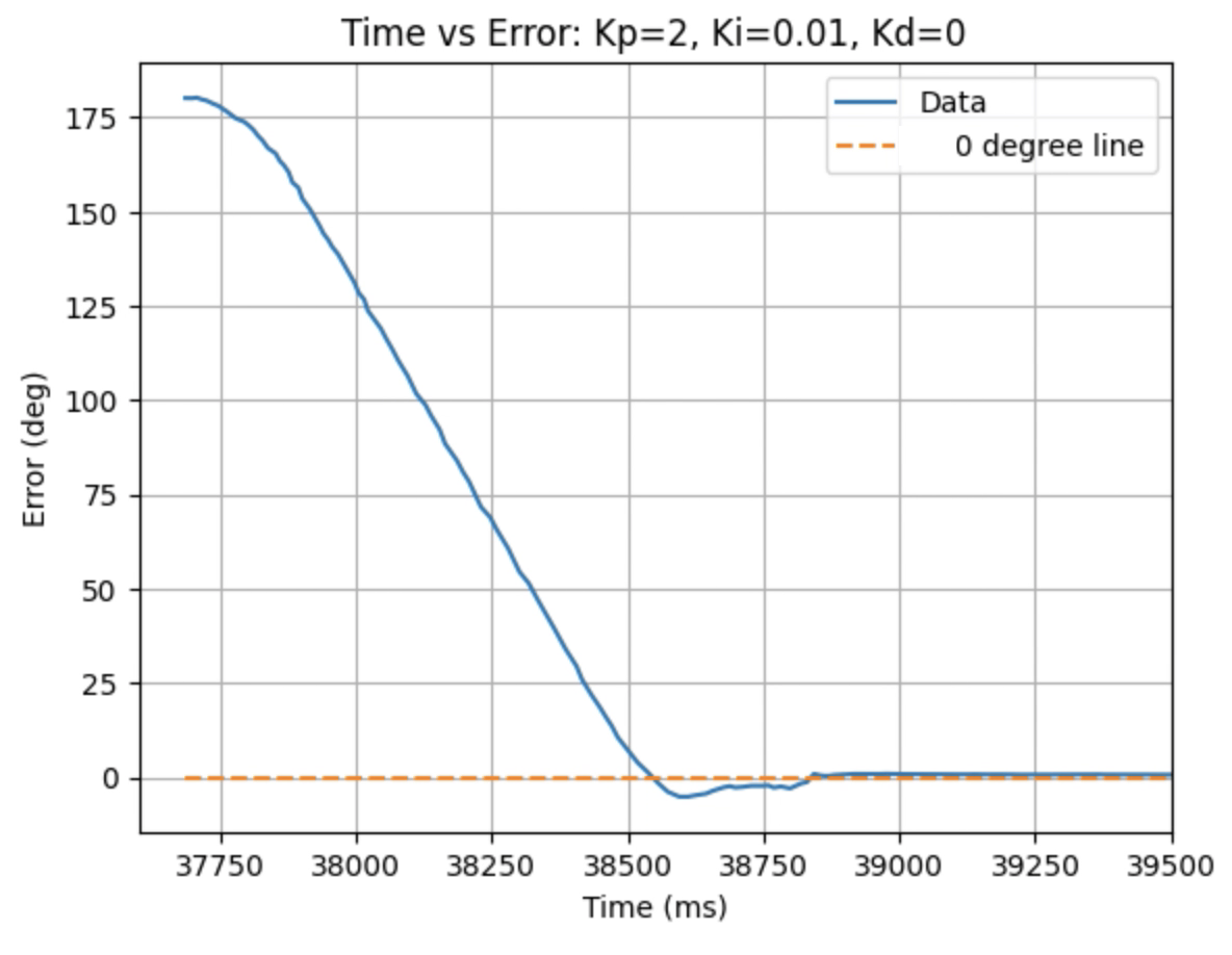
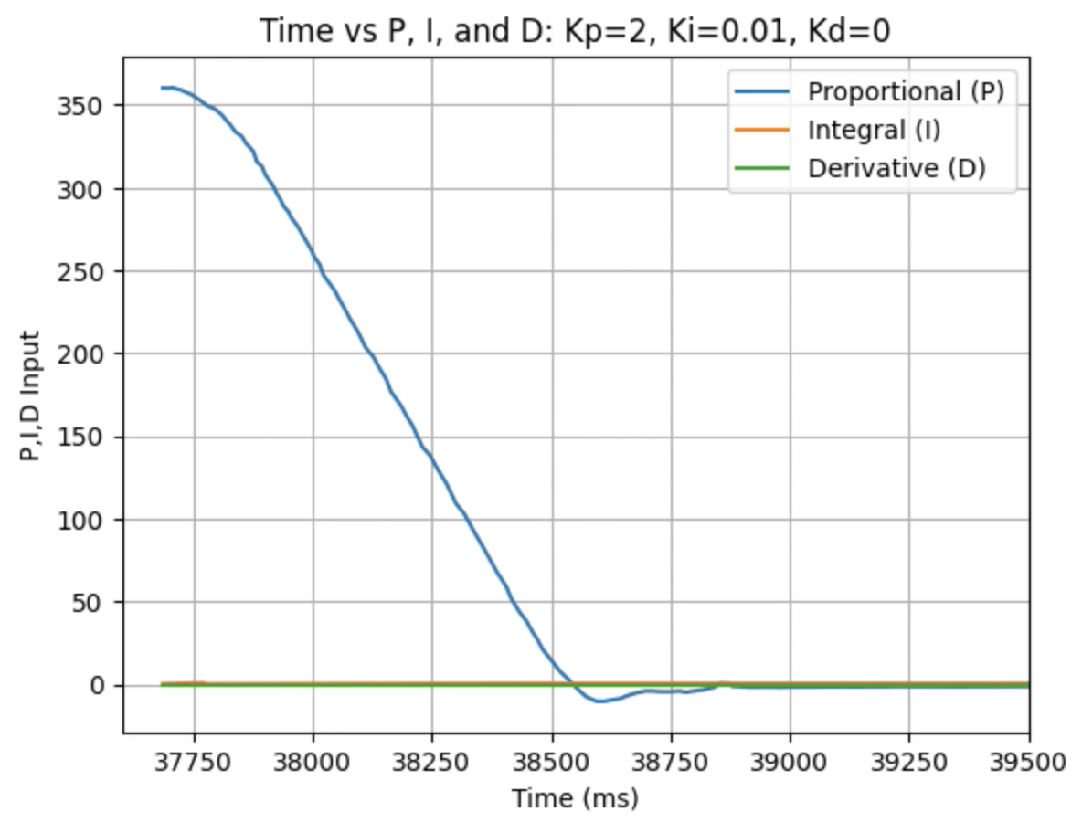
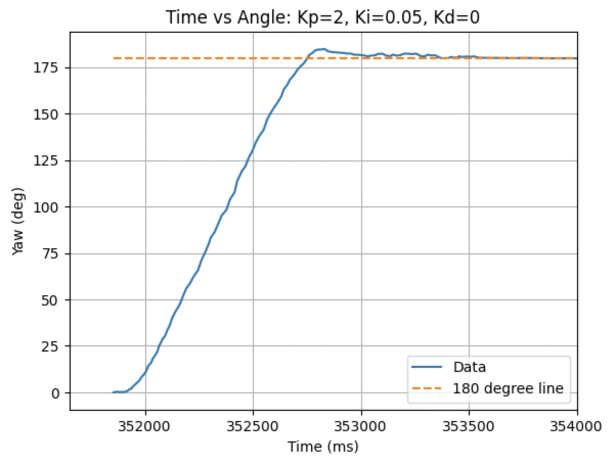
Below are graphs for the tested values for Kp and Ki.
Graphs for Kp = 2 and Ki = 0.01:

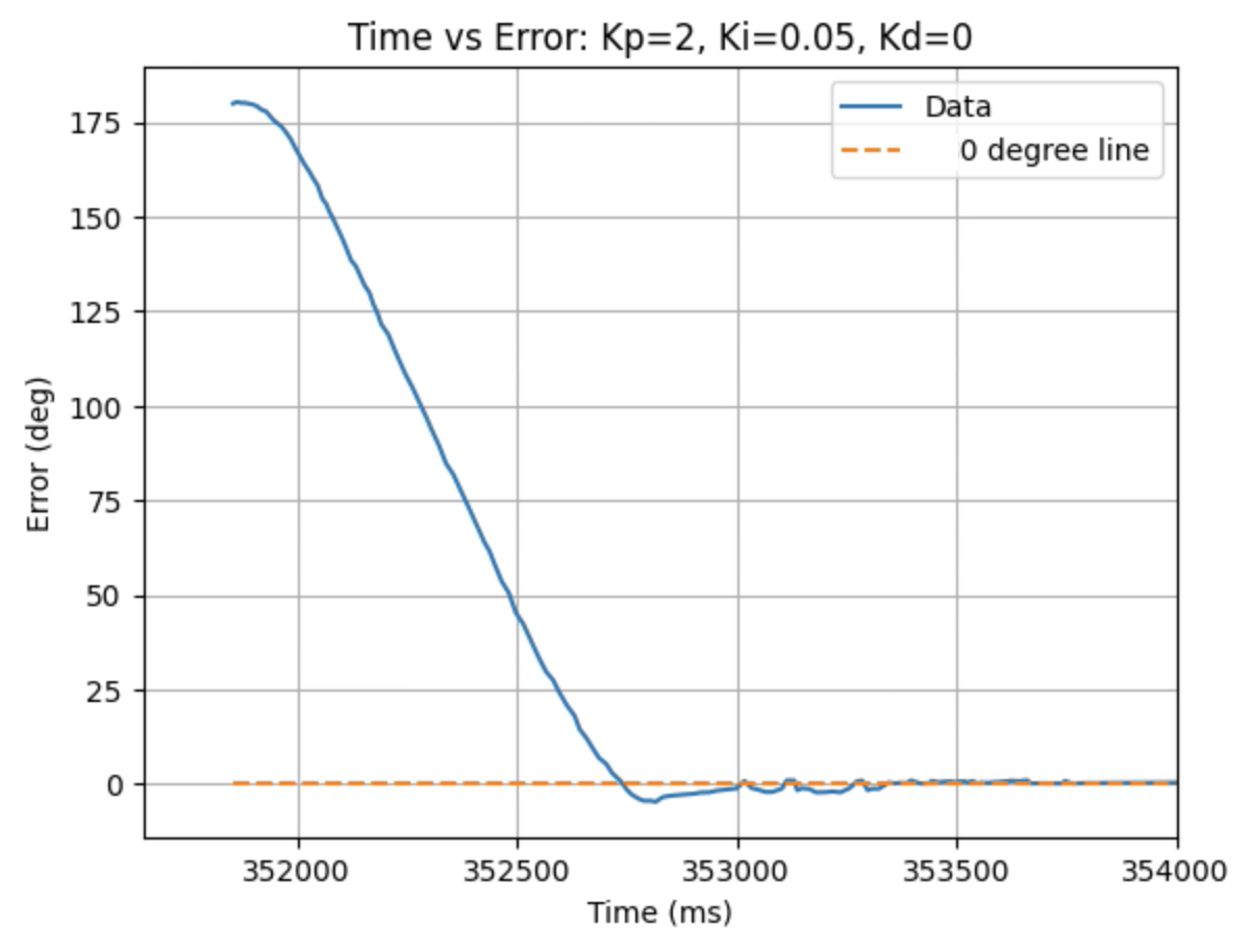
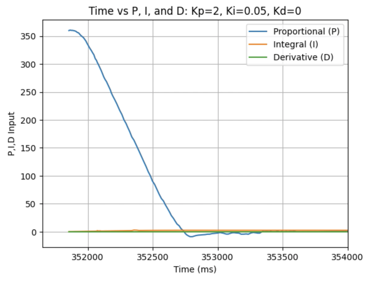
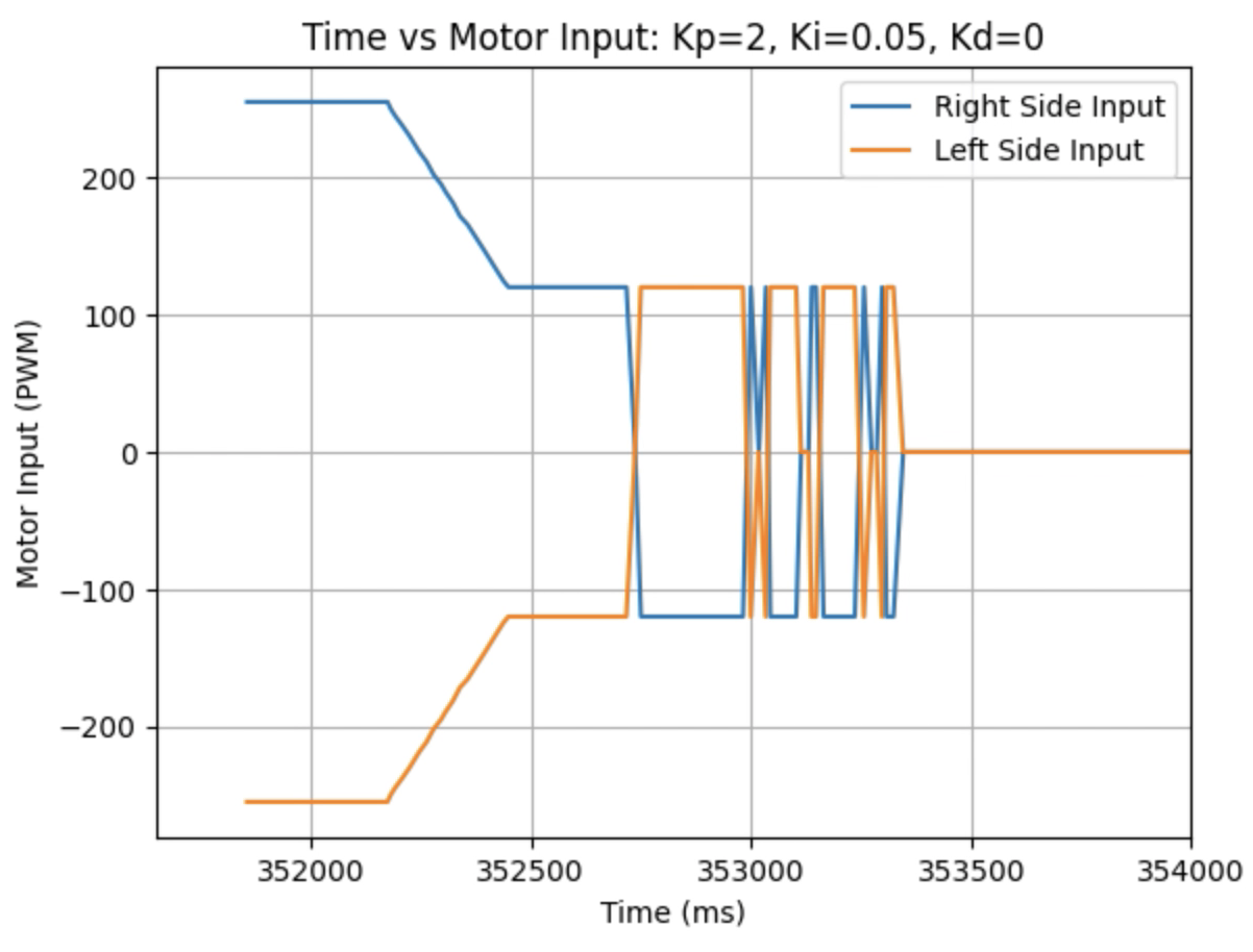
Graphs for Kp = 2 and Ki = 0.05:
Graphs for Kp = 2 and Ki = 0.1:
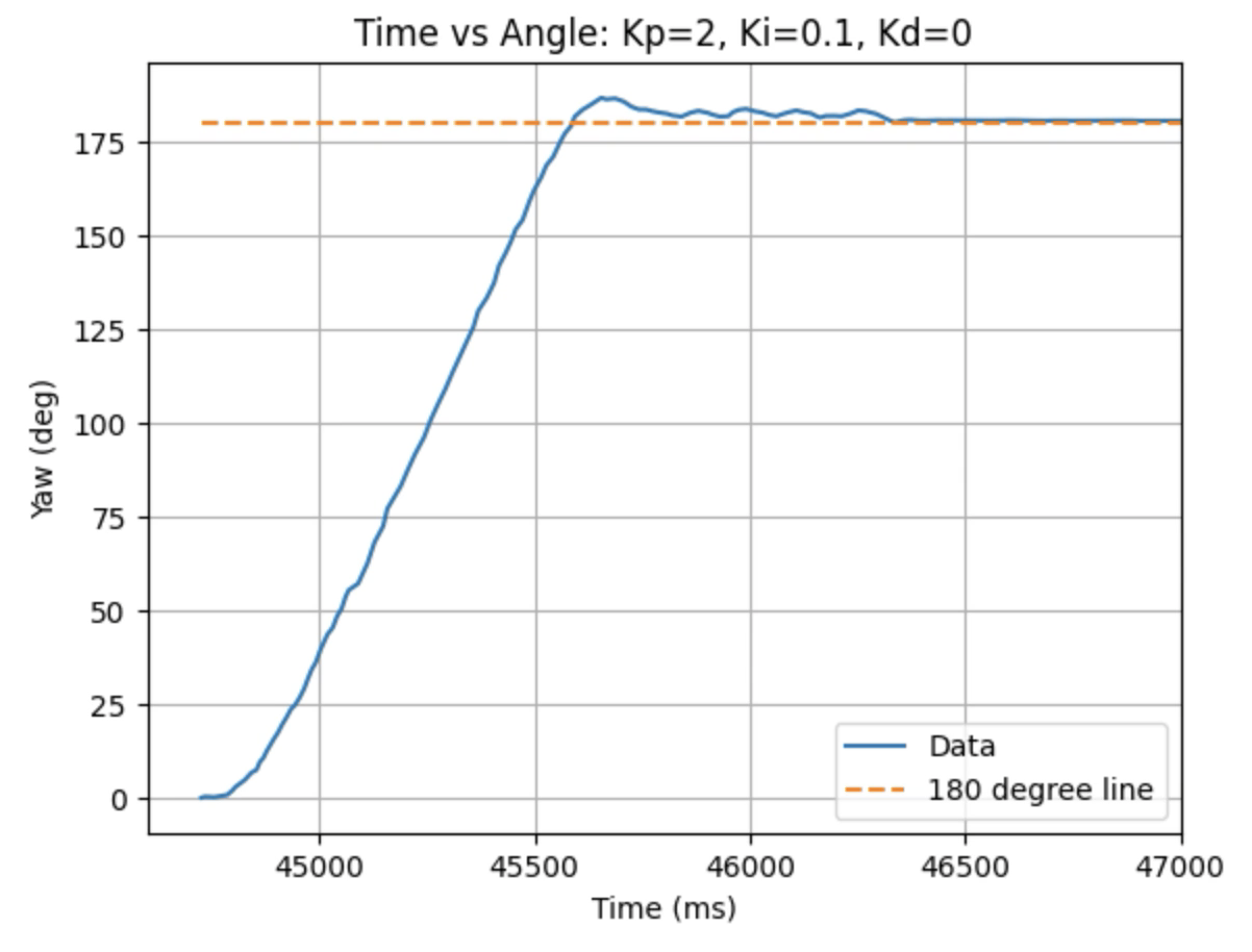
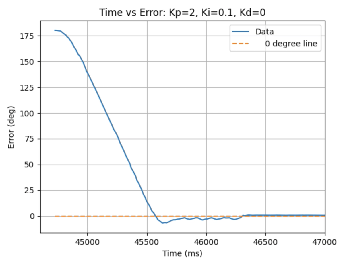
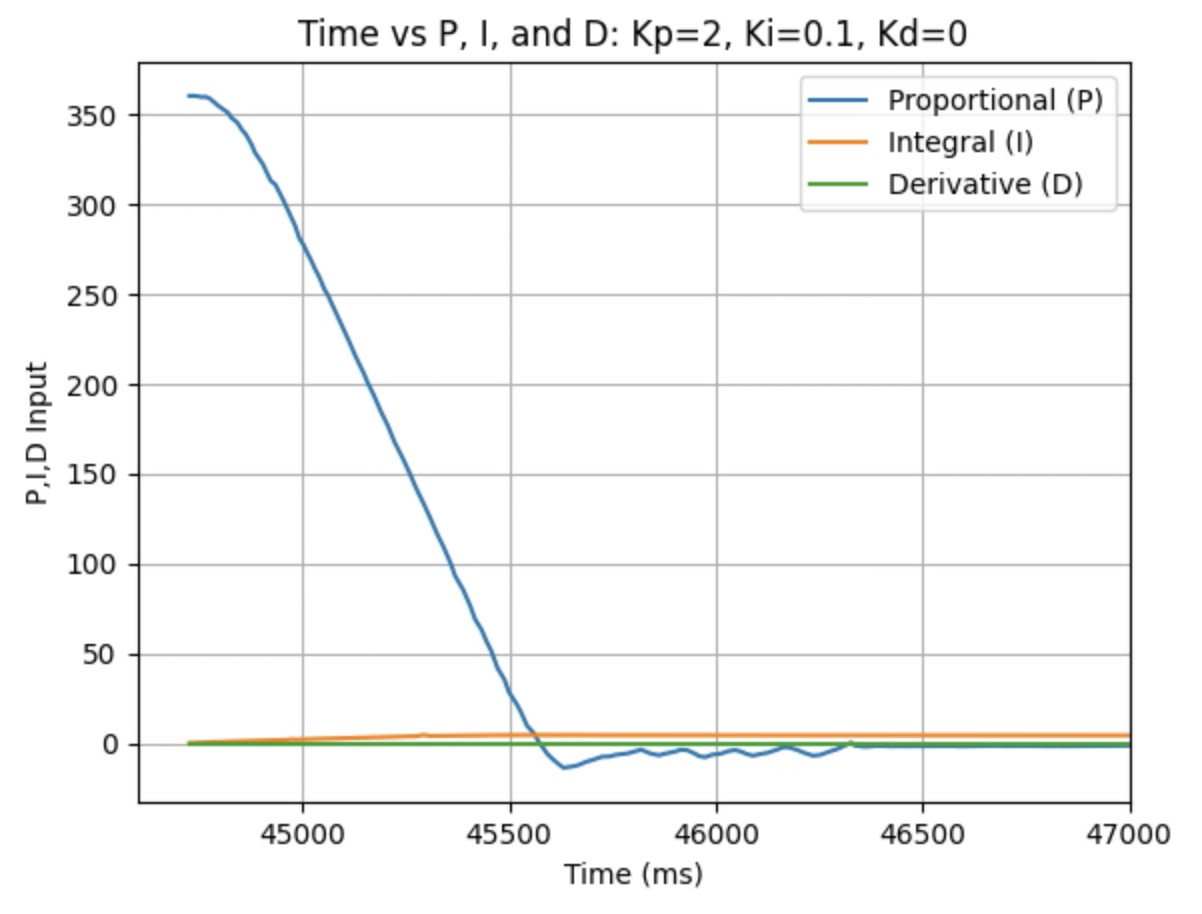
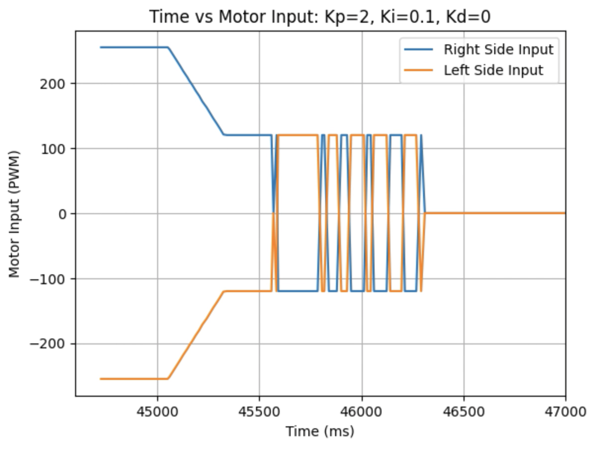
Graphs for Kp = 2 and Ki = 0.2:
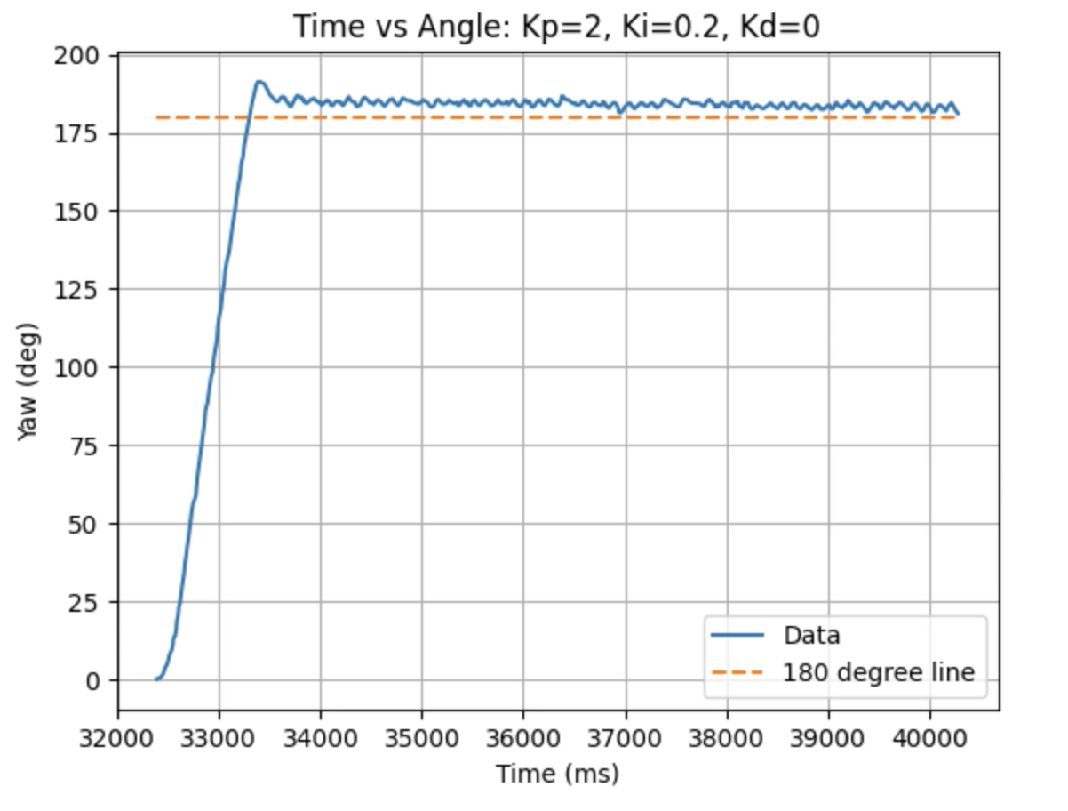
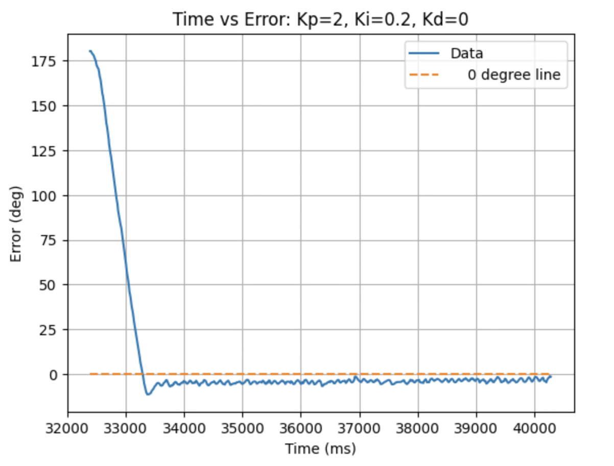
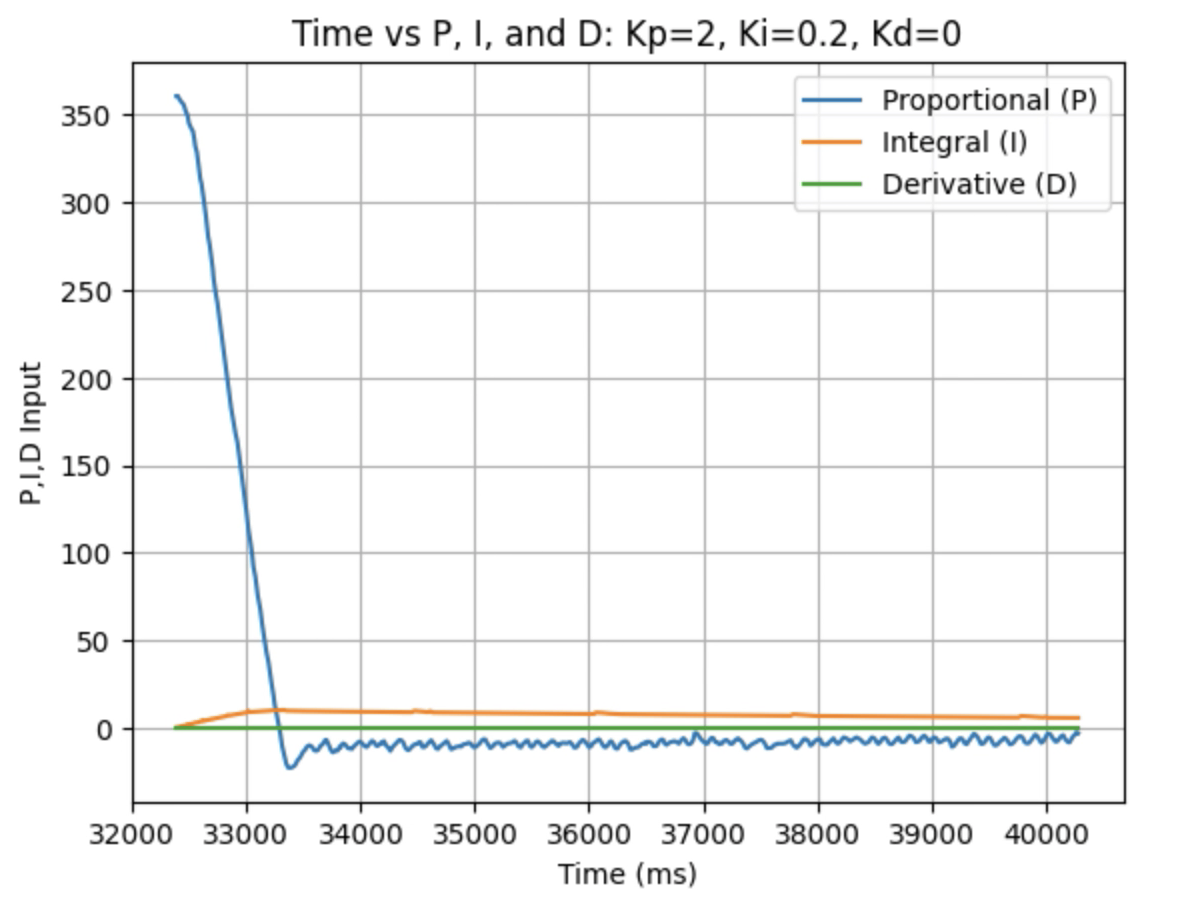
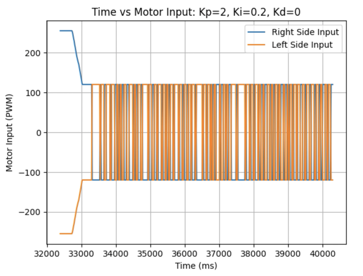
Trends that can be observed include, as the value for Ki increases the amount of oscillation and overshoot of the robot at the desired angle increases. The motor input for all tested values starts at the maximum of 255 before decreasing to a value of 120 before reaching the desired angle. For a value of Ki = 0.01 there is minimal overshoot and oscillation and a value of Ki = 0.05 also results in minimal overshoot but slightly more oscillation. For Ki = 0.1 there is more oscillation before reaching the desired angle and for Ki = 0.2 the oscillation continues for a longer amount of time. I choose a value of Ki = 0.05 to move on to testing the proportional, integral, and derivative controllers together.
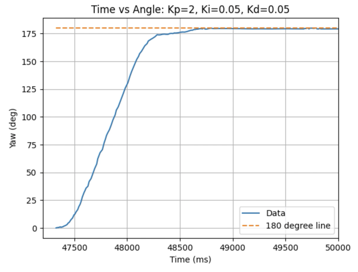
The next step involved finding the value for the derivative constant Kd to remove overshoot at 180 degrees. I initially calculated the derivative using the following code (line 15): This resulted in a large spike for the first derivative control calculation as well as some noise as can be seen in the plotted graph for Kd = 0.05 below:
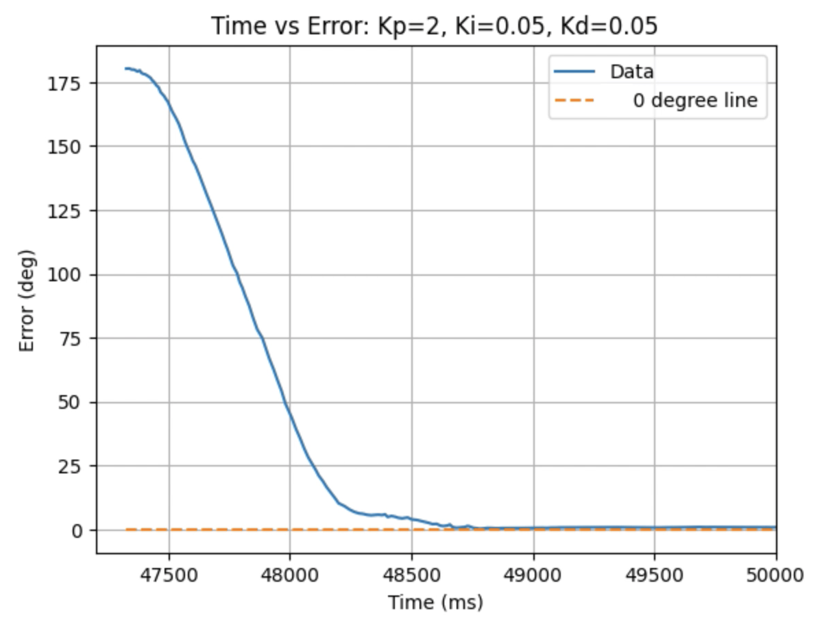
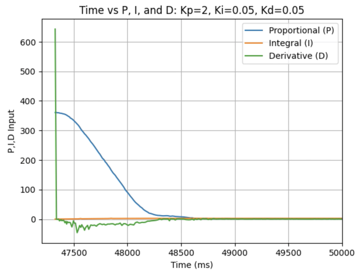
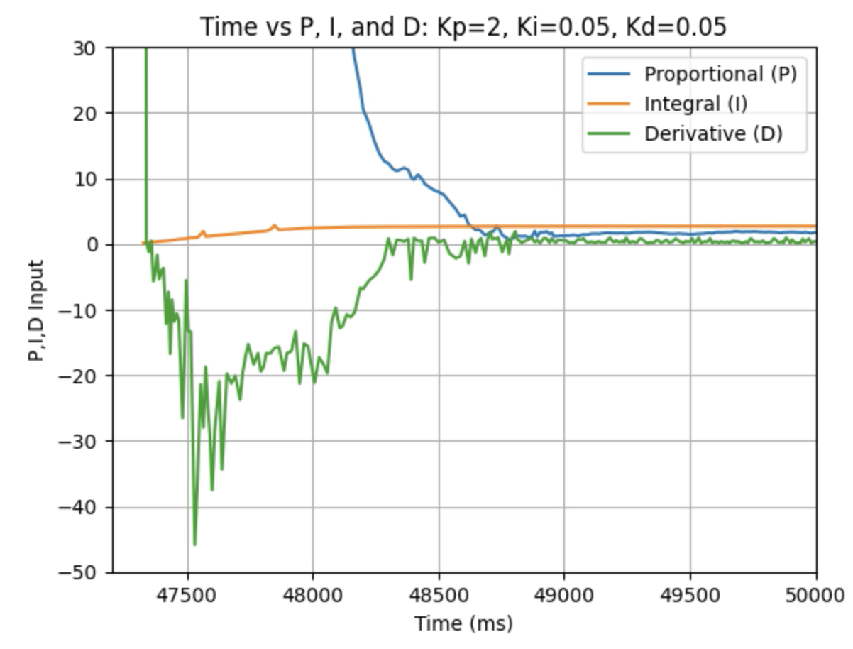
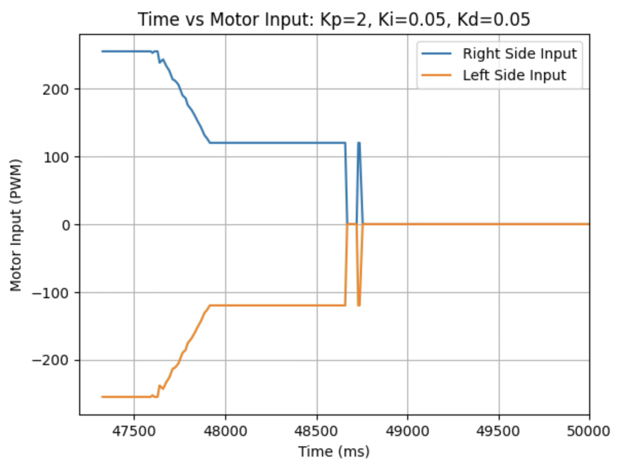
After observing the previous graphs and to prepare for changing the setpoint in real time, I changed how the derivative control component was calculated. I used the information on this website. Instead of calculating the derivative of a signal using the integral of another signal, I calculated the derivative using the Z output of the gyroscope using the following code: This resulted in the large spike being removed, but there was still some noise in the derivative controller as can be seen in the plotted graph for Kd = 0.08 below:
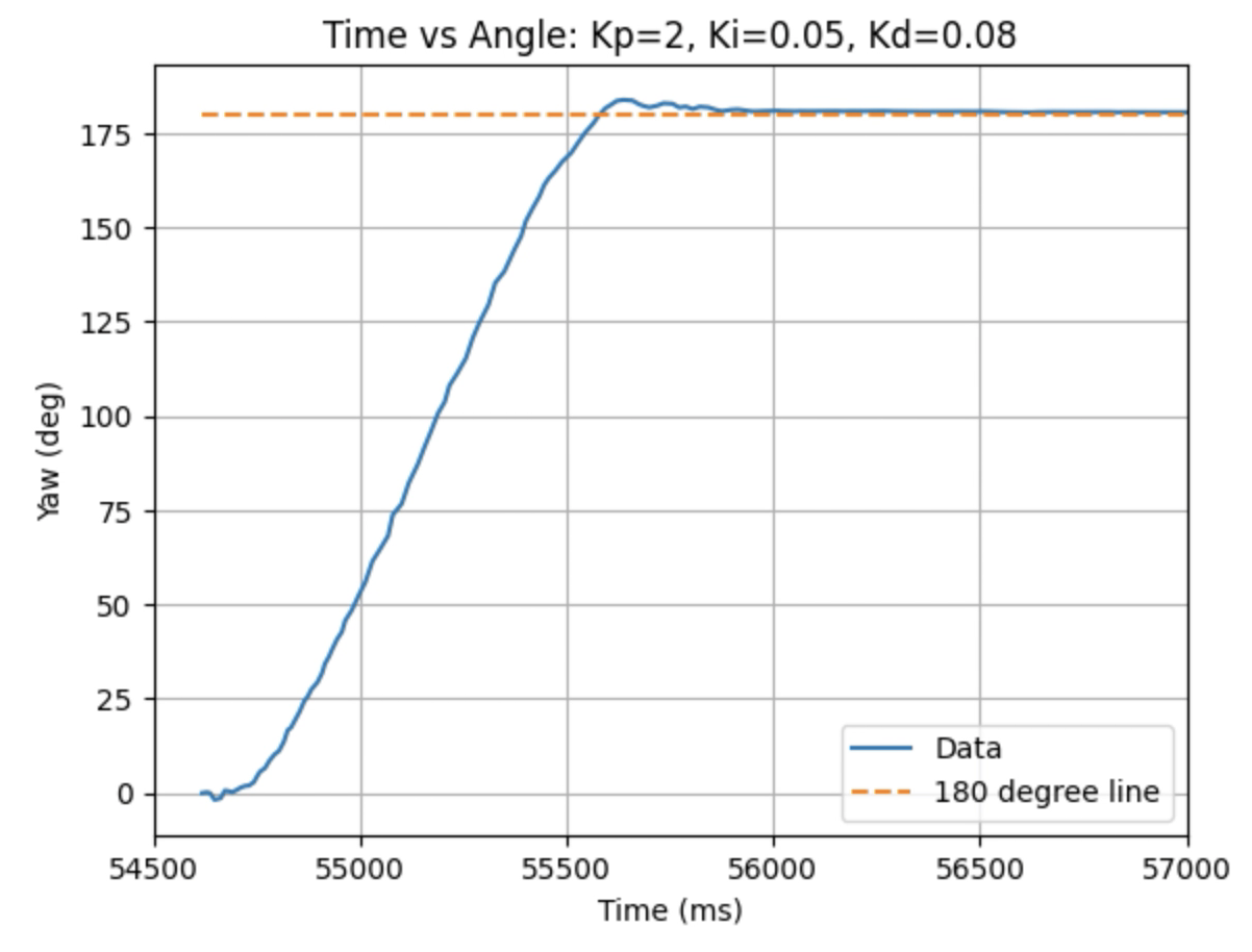
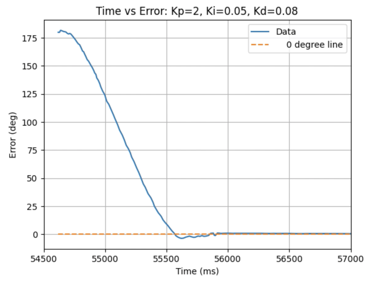
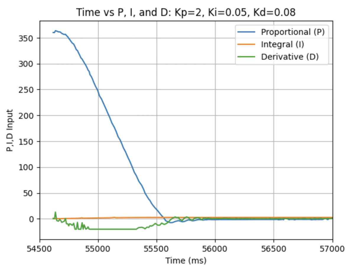
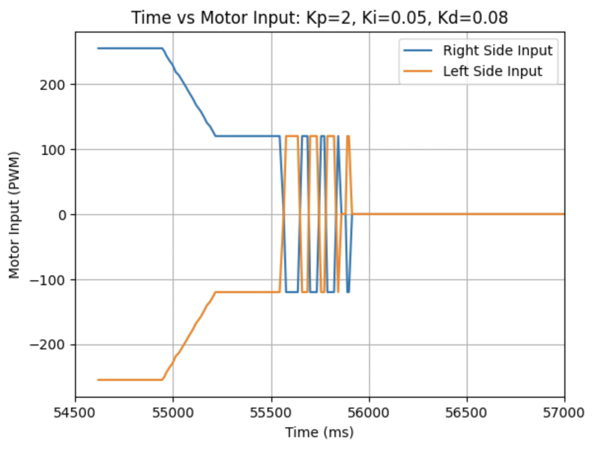
The final derivative calculation used the previous gyroscope output combined with a low pass filter with an alpha of 0.3055 to remove some of the noise. The calculation for alpha is found below along with the final code to find the derivative control.

I tested a serives of Kd values to find where the overshoot was reduced. The final derivative calculation resulted in the spike and the noise being removed as can be seen in the below graphs.
Graphs for Kp = 2, Ki = 0.05, and Kd = 0.03:
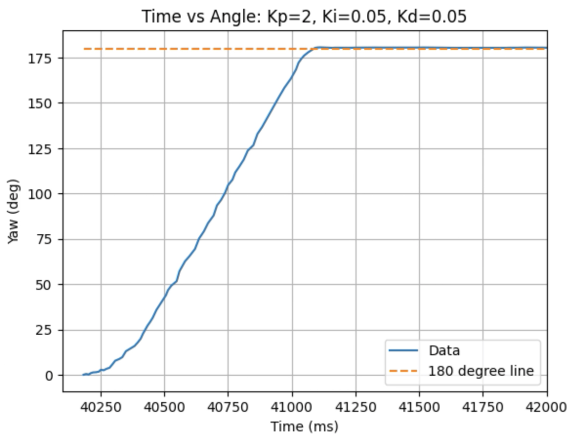
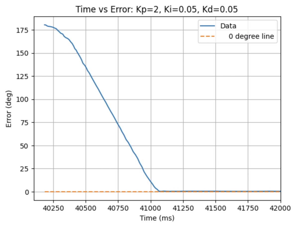
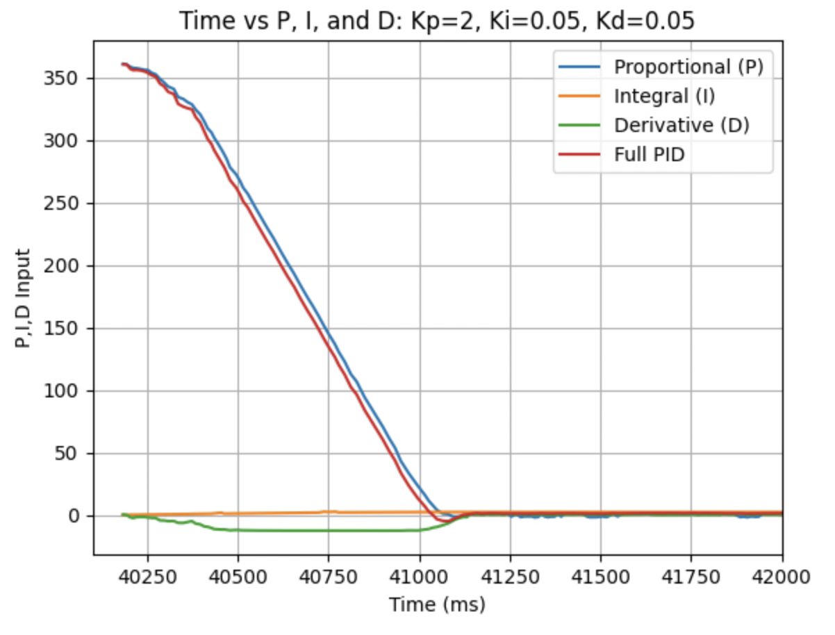
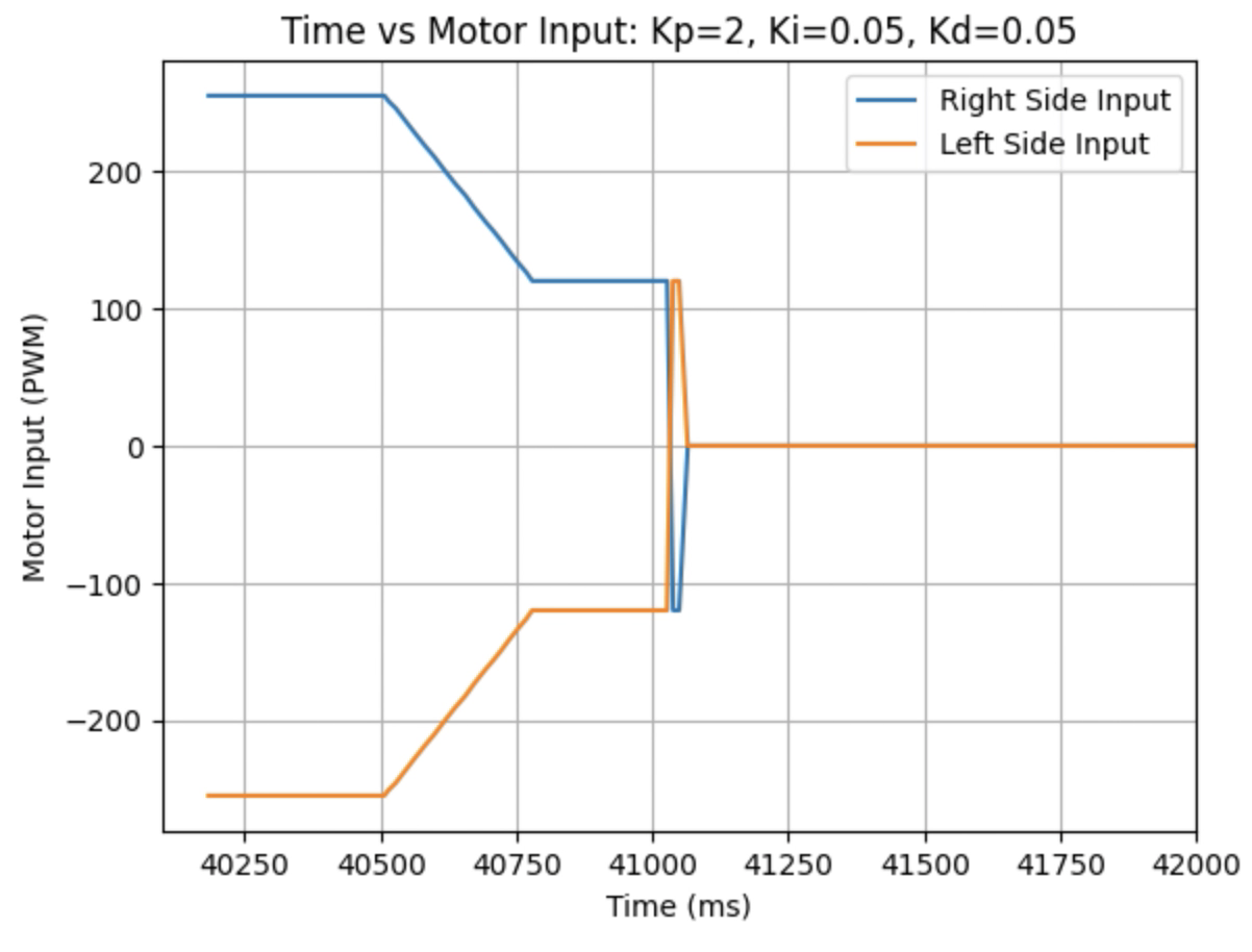
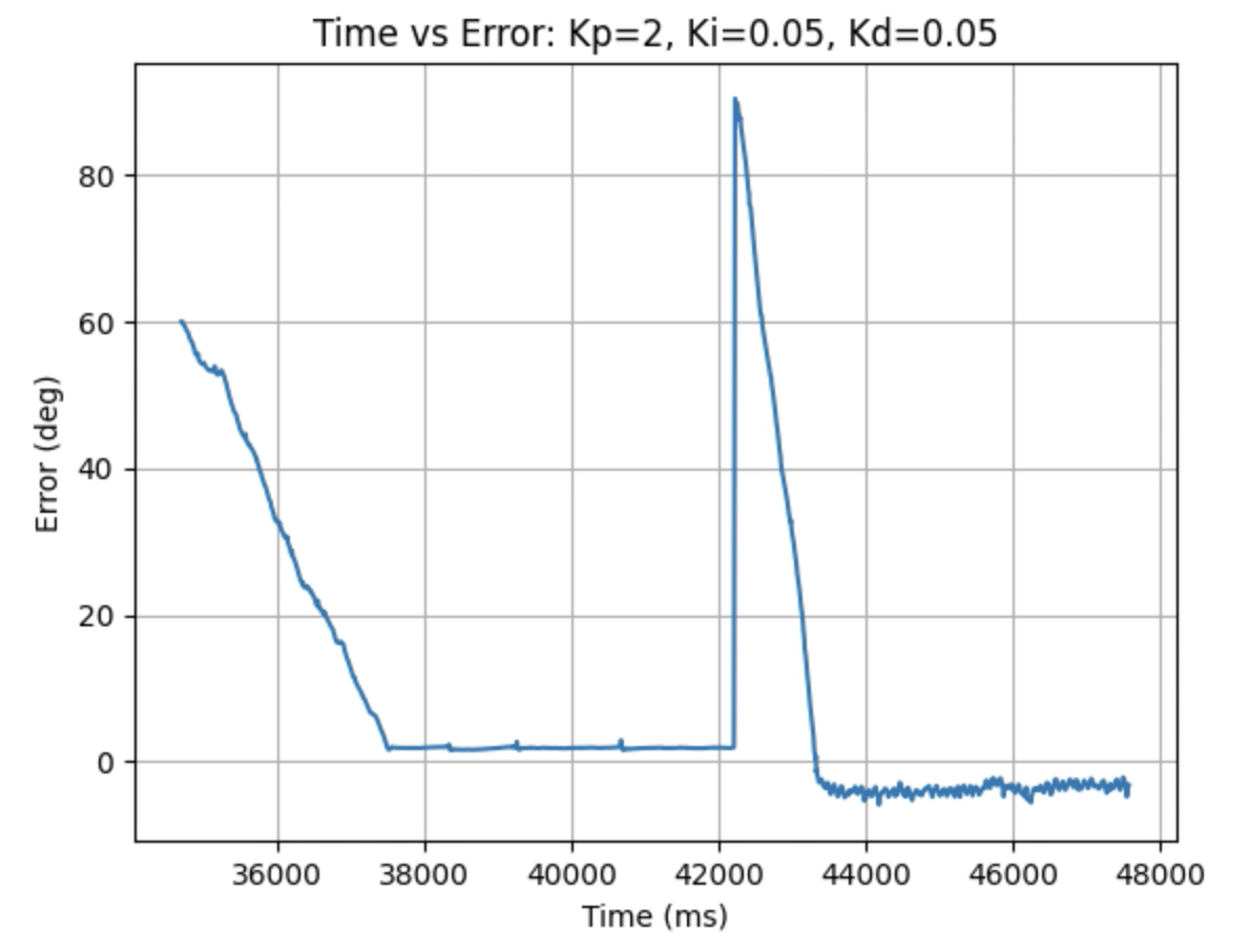
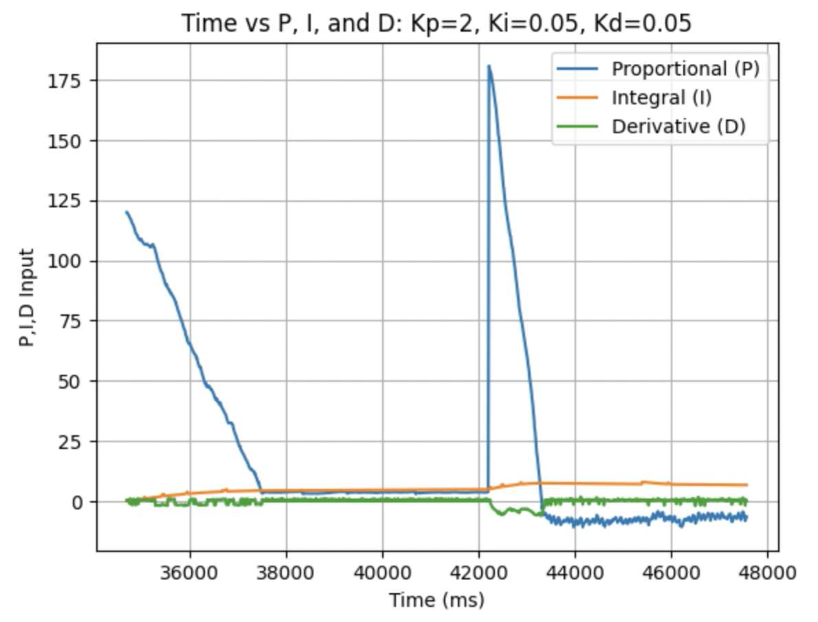
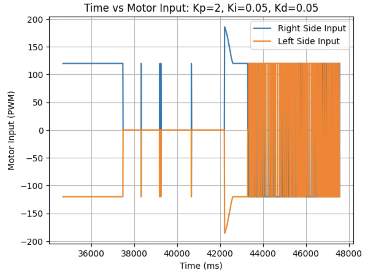
Graphs for Kp = 2, Ki = 0.05, and Kd = 0.05:
Graphs for Kp = 2, Ki = 0.05, and Kd = 0.06:
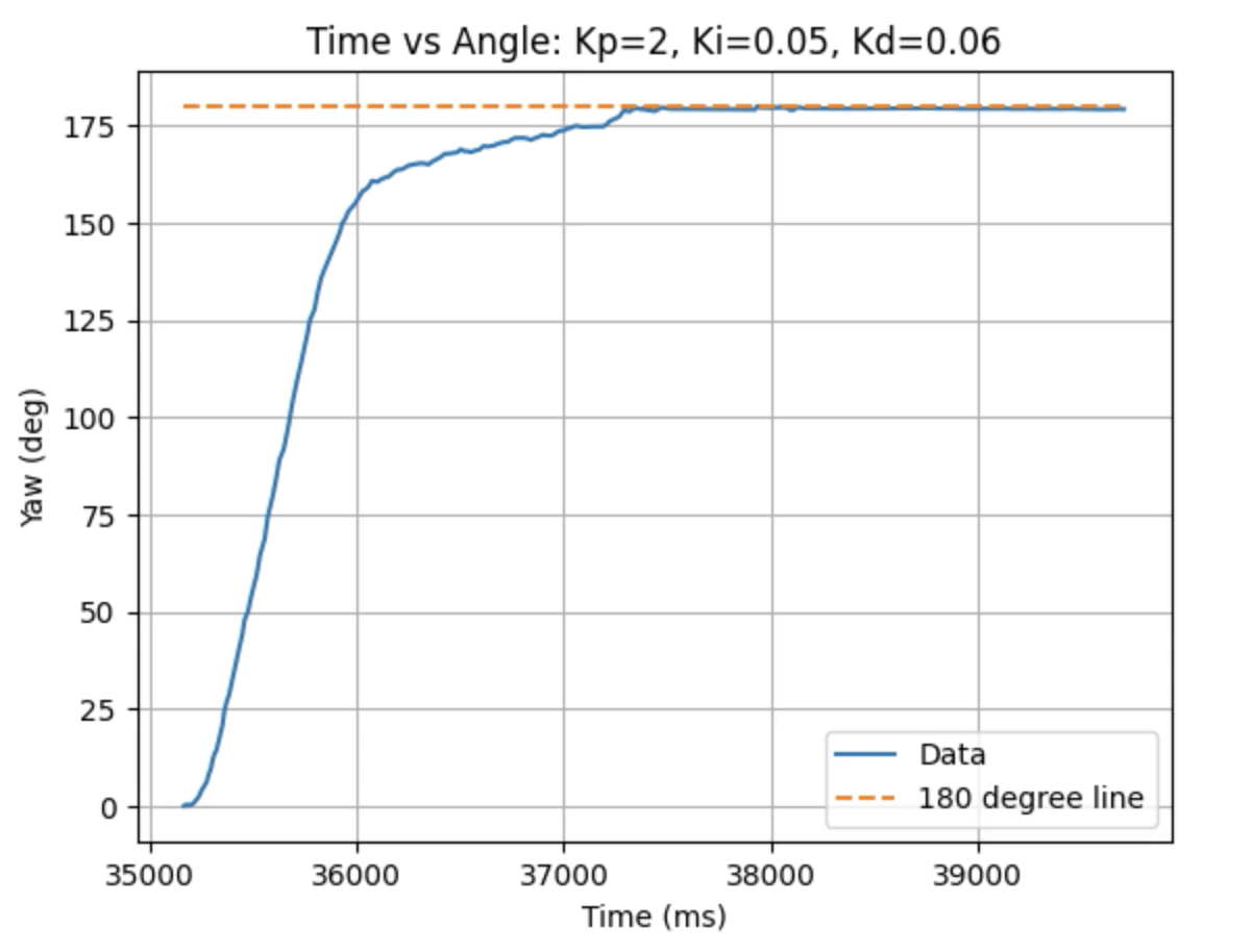
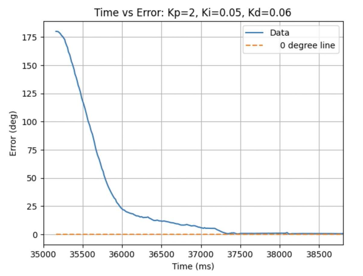
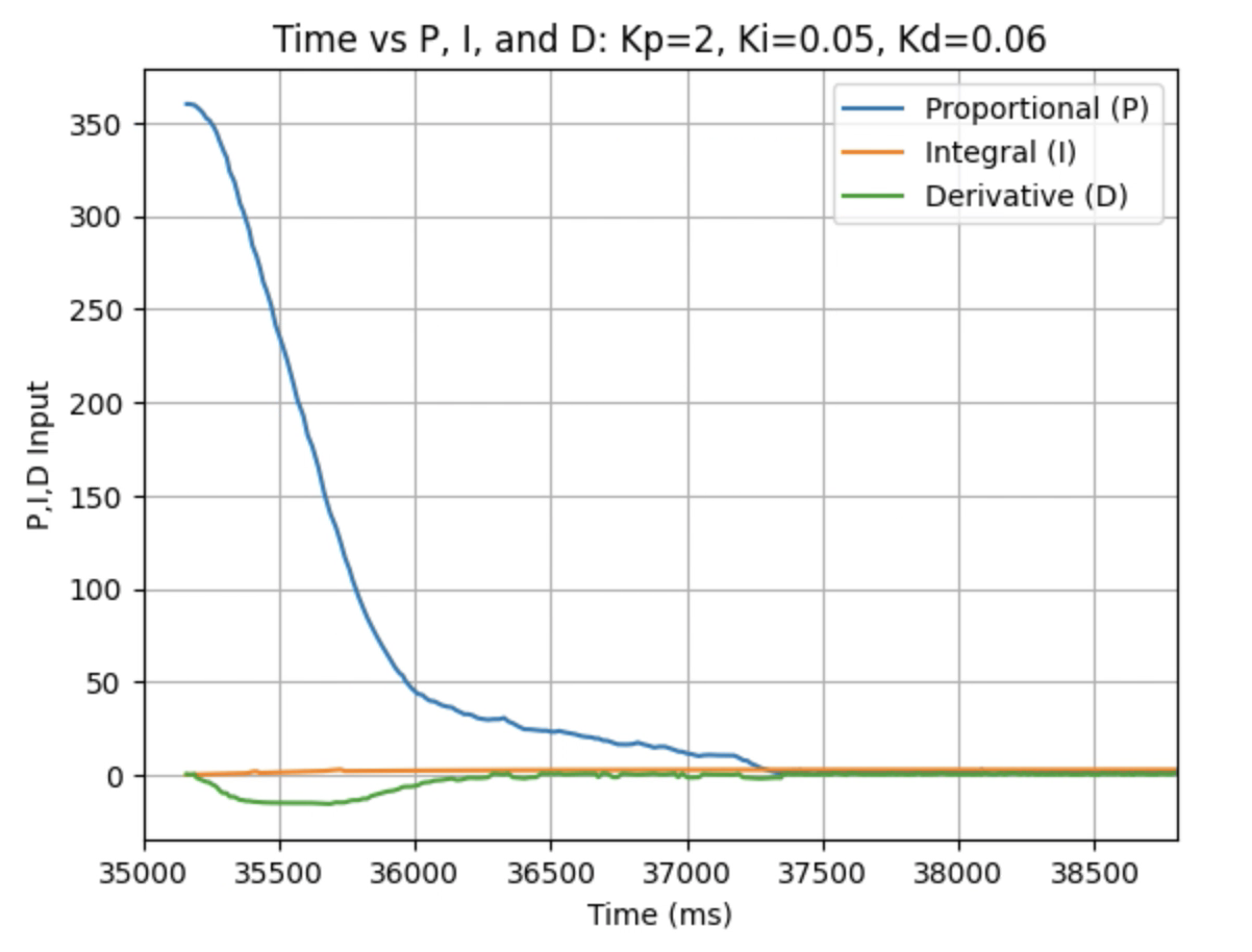
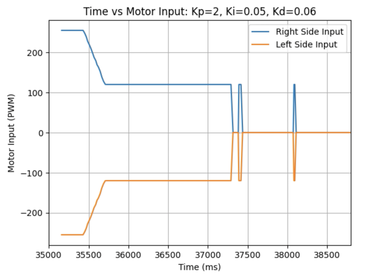
Graphs for Kp = 2, Ki = 0.05, and Kd = 0.08:
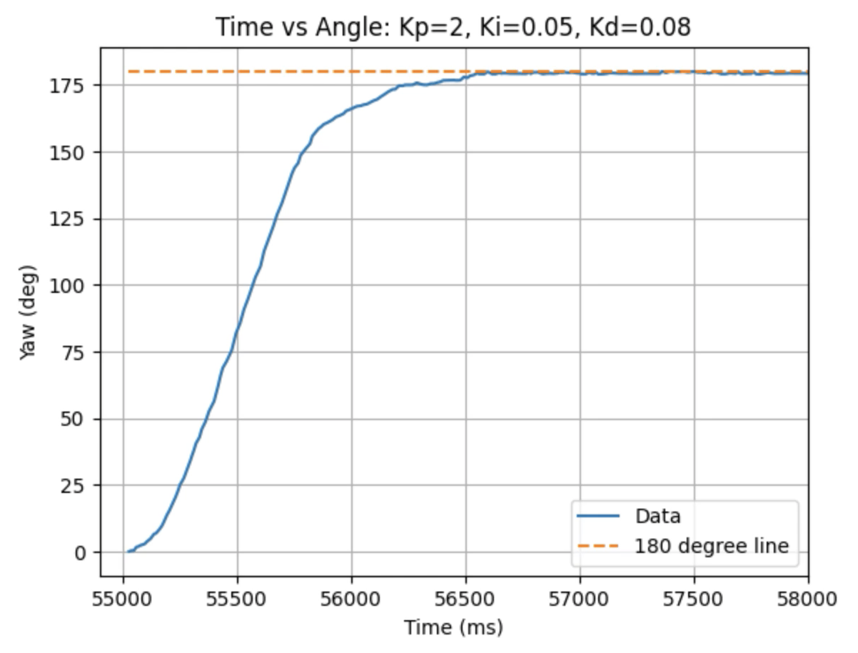
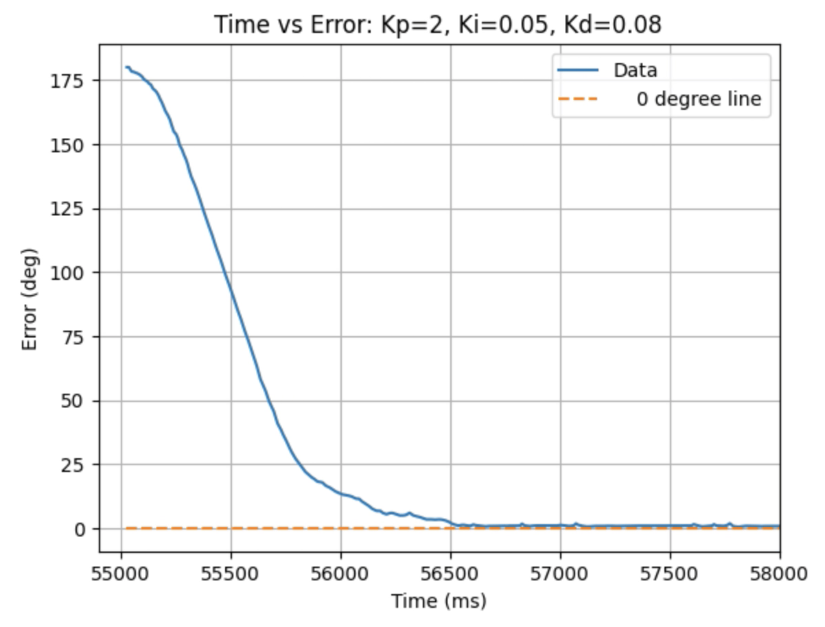
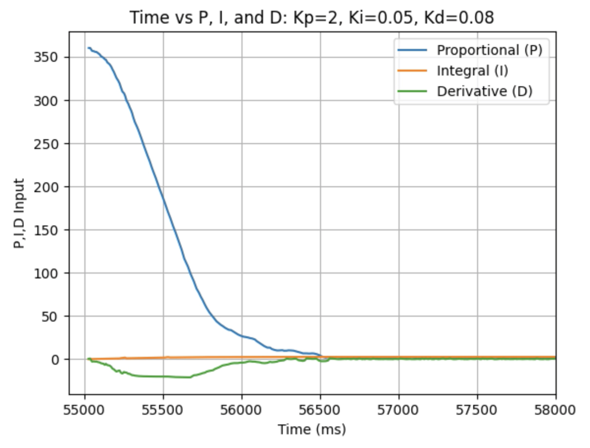
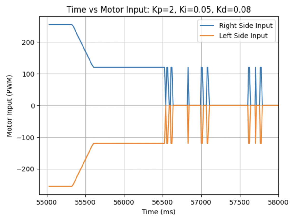
I choose a final value of Kd = 0.05 as the robot did not overshoot the desired angle of 180 degrees.
Below is a video of the robot turning +180 degrees at Kp = 2, Ki = 0.05, and Kd = 0.05:
Below is a video of the robot at 0 degrees:
I also tested negative angles. Below is a video of the robot turning -90 degrees:
After tuning the PID controller I tested changing the setpoint (desired angle) while the controller was running and recording data for multiple changed angles. During the first few attempts the data was not entirely recorded correctly as can be seen in the below graphs.
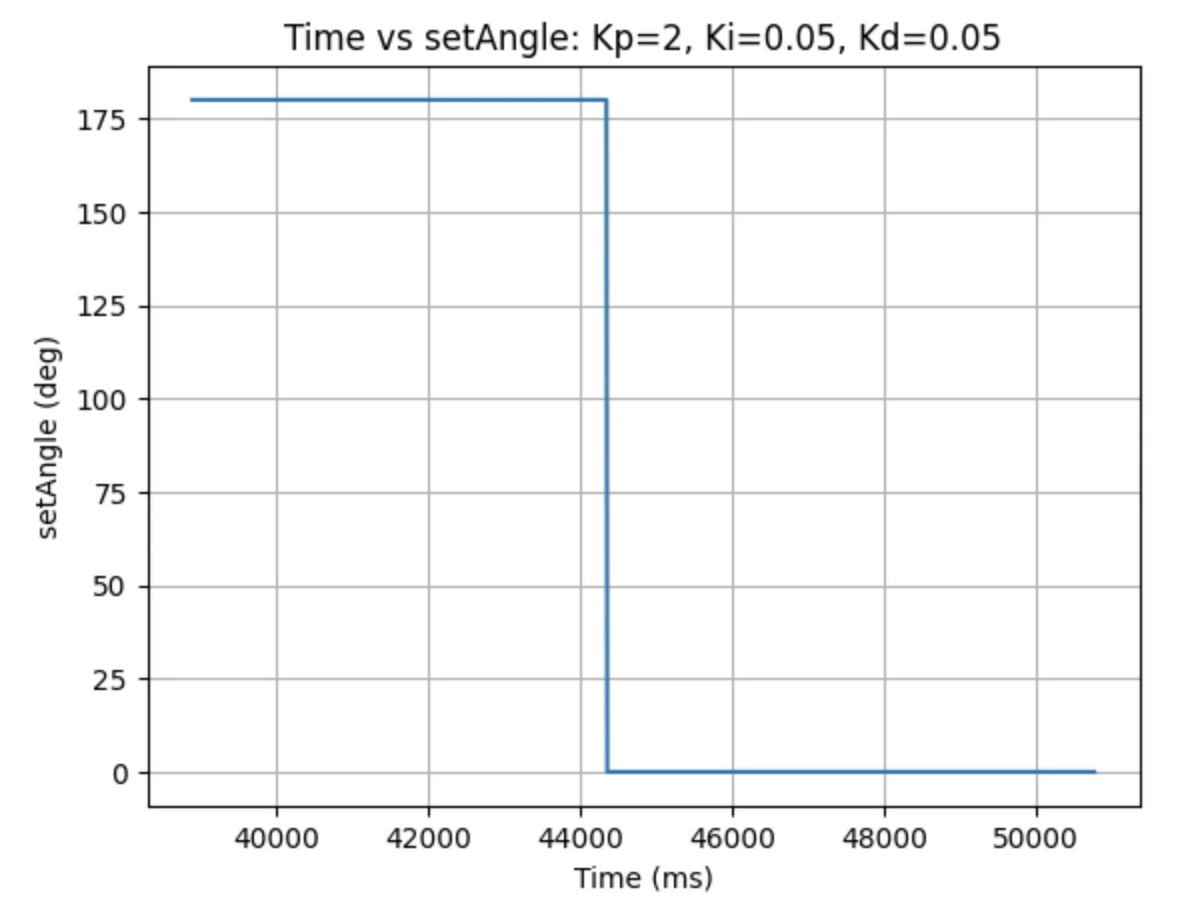
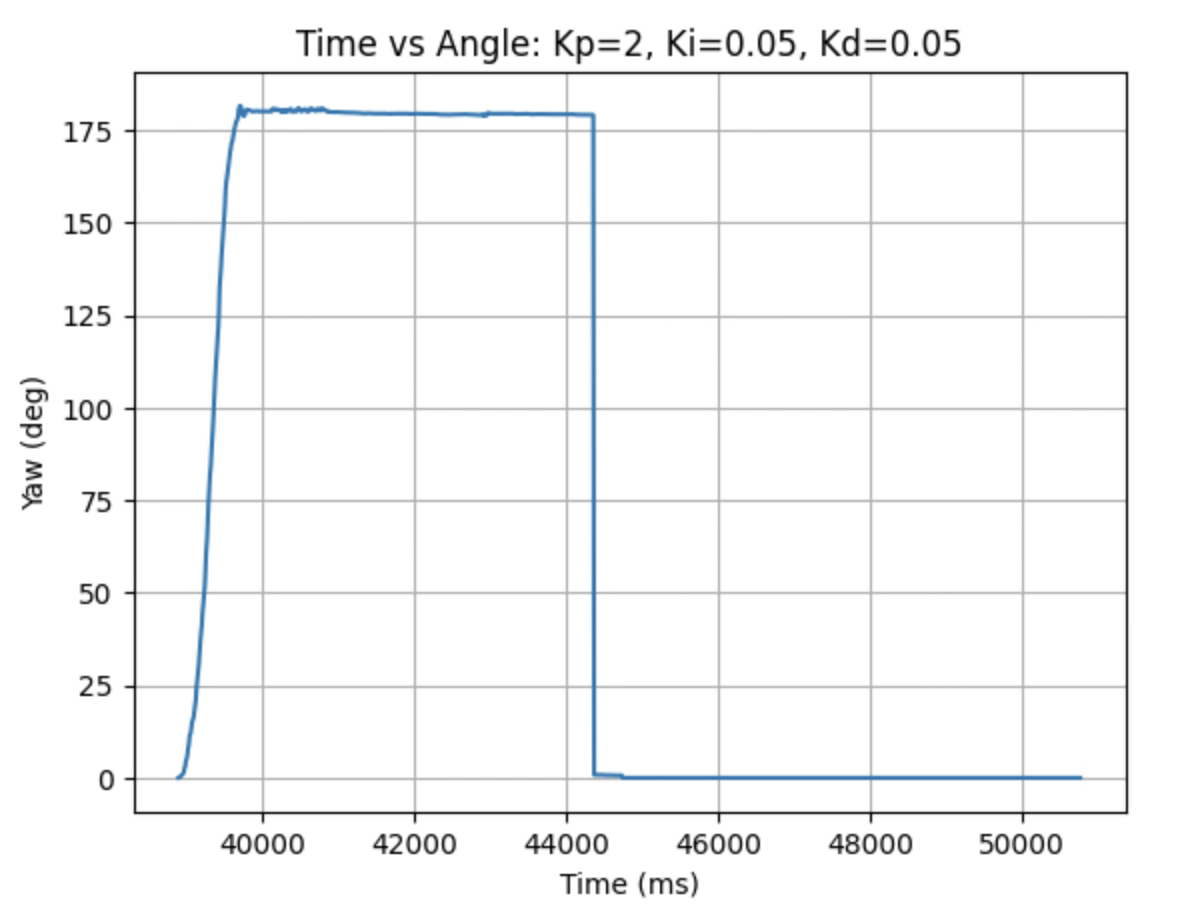
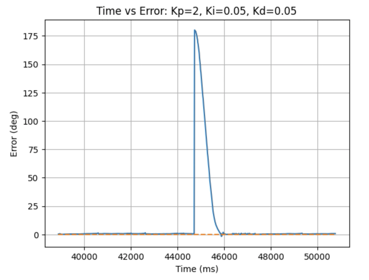
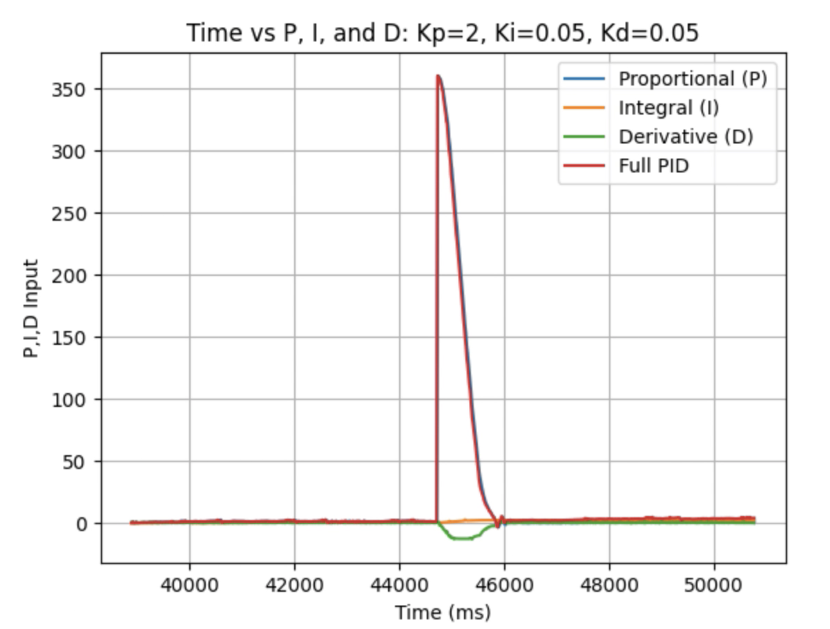
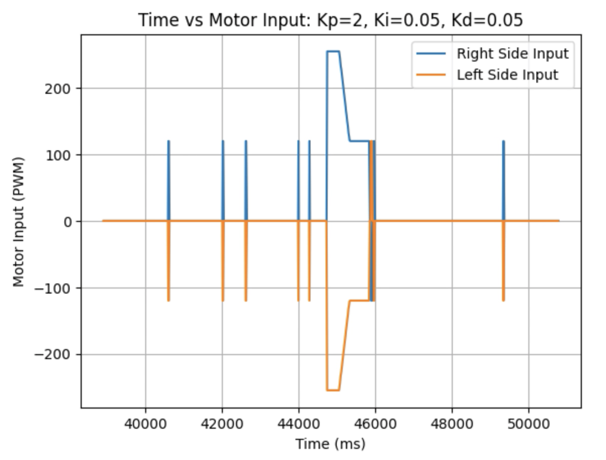
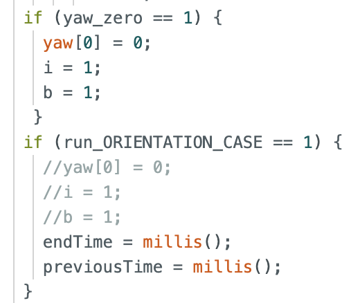
I realized that whenever I changed the angle the array indices changed for recording yaw. To address this issue I added another if statement in the Arduino case ORIENTATION_CASE that allowed me to control when to set yaw to zero and when to set the initial indicies for the array's to one. The changed and added code can be found below.
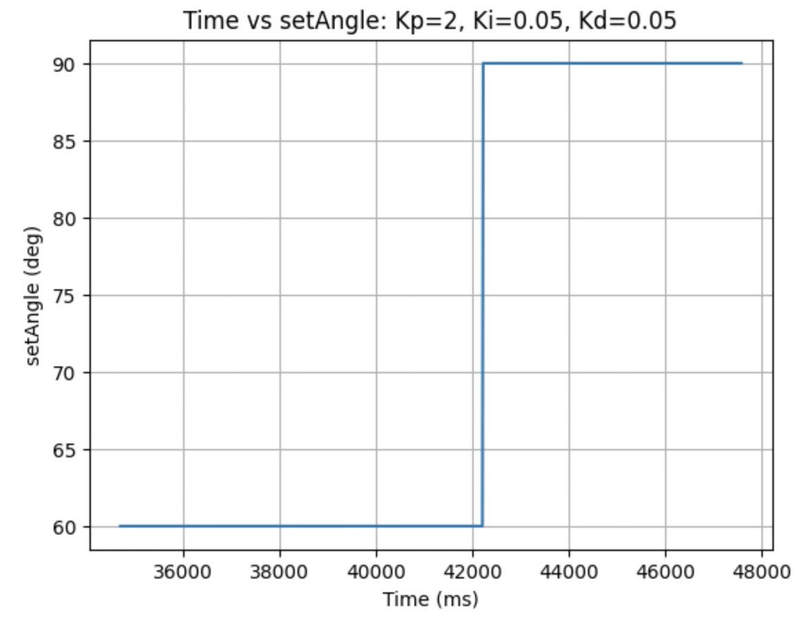
The example below shows a change of 60 degrees to 90 degrees:
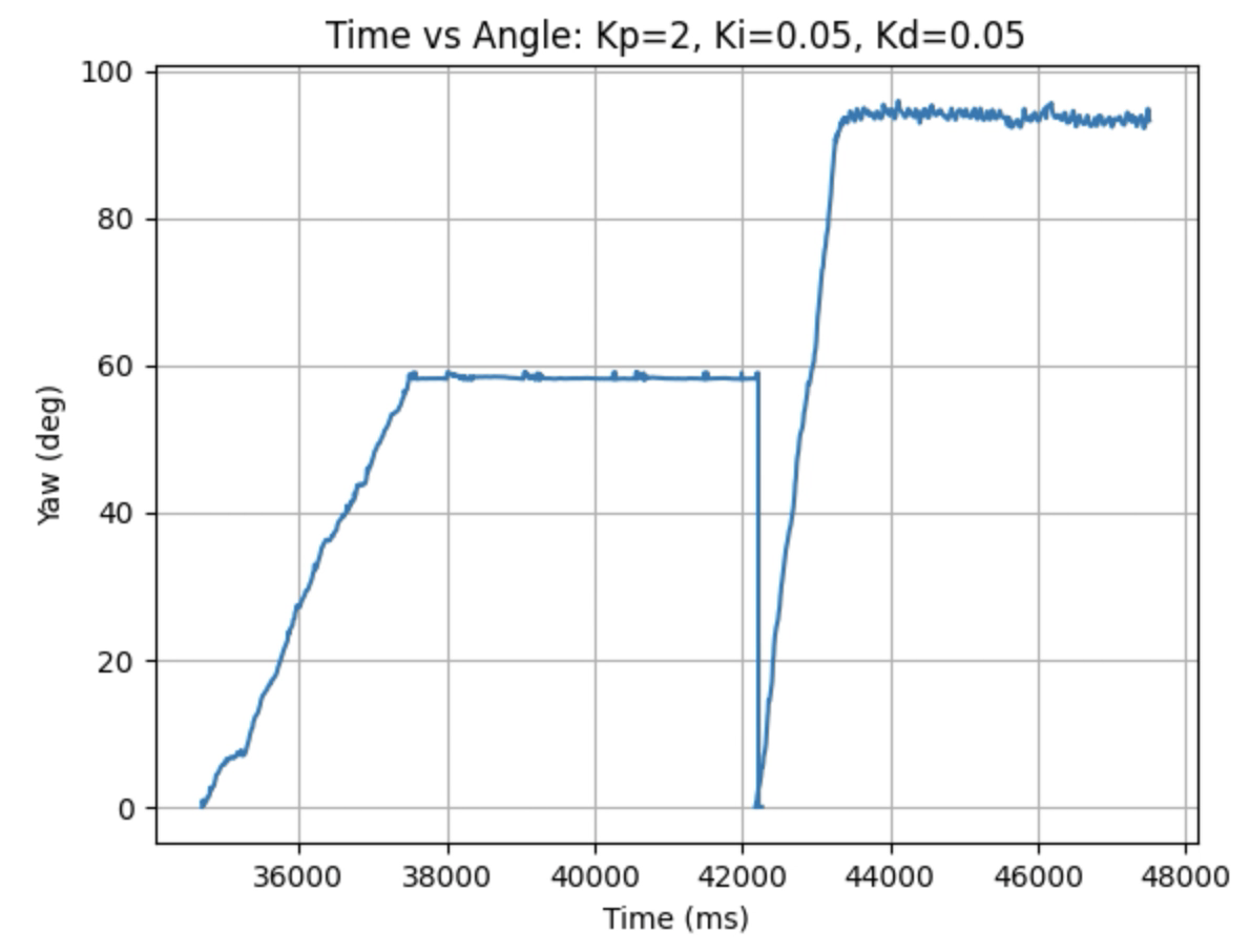
I was able to record data for multiple angle changes.
For future navigation and stunts, I might need to change the setpoint in real time depending on the desired task. For this lab changing the setpoint was done through Jupyter Notebook, but changing the setpoint could also be done through a series of if statements in Arduino IDE. Changing the setpoint may be beneficial during navigation along with using data from the ToF sensor readings to navigate through the course.
The full PID controller with wind up protection, as described earlier, can be observed in the videos below.
Robot turning +90 degrees on carpet:
Robot at 0 degrees on carpet:
The PID controller works on multiple surfaces when maintaining an angle. When turning towards an angle there is slightly more delay compared to on a flat surface, but the robot is still able to reach the desired angle. Below is a video showing the serial monitor outputs for the wind up protection. In the video the KiIntegral term increases over time until reaching 200 and then does not further increase.
The robots orientation can be controlled while driving by altering the Arduino IDE code from the previous Lab 5 for the functions FORWARD and BACKWARD. As the robot drives either forward or backward the desired yaw angle will be set to zero. If the yaw angle changes from zero the PID controller will be used to increase the PWM of one wheel side and decrease the PWM of the other wheel side in order to keep the robot moving straight. For longer runs the gyroscope drift may be needed to accounted for. In the below video the yaw drifts from 0.01 to -8.72 degrees over (27.299 - 04.300) = 22.999 seconds,which is around -0.3796 degrees per second.
See above: Completed previously.
Thank you to all of the TAs that answered my questions. I referenced the past lab reports of Liam Kain, Rafael Gottlieb, Larry Lu, Julian Prieto, and Ignacio Romo.
The objective of the lab to to gain experience working with PID controllers. I am a 5000 level student and I choose to work on a PID controller. Labs 5-8 detail PID, sensor fusion, and stunts. This lab is focused on using a PID controller for position control of the robot. Lectures 6, 7, and 8 were consulted during the lab.
The used lab materials include:
For this lab a PID controller will be used for position control of the robot. The below equation from the course Lecture 7 is used to compute the value for the PID controller:

This equation uses the error e(t) (difference between the final desired value and the current value) in proportional, integral, and derivative control to calculate the new PID input value u(t). For this lab the error is the difference between the desired distance from the wall (1ft) and the robots current distance from the wall. The calculated PID input value is related to the robots speed. Proportional control multiplies a constant Kp by the error. Integral control multiplies a constant Ki by by the integral of the error over time. Derivative control multiplies a constant Kd by the rate of change of the error.
During the Prelab, I determined how to send and receive data over Bluetooth. Two Arduino IDE cases were initallized. The case PID_CASE starts and stops the PID controller and the case SEND_PID_DATA sends the collected PID data to Jupyter Notebook. The PID controller starts when a command from Jupyter Notebook is run. The command inputs include a start(1)/stop(0) value; the desired setDistance value to determine the desired end distance from the wall; and the Kp, Ki, and Kd constant values. In Jupyter Notebook a notification handler similar to the notification handler from Lab 1 is used to create the data array. The PID controller stops when the first input value is set to zero.
I also determined what data I wanted to store and send to Jupyter Notebook. Initially, I stored time, two ToF distance values (one in millimeters and one in feet), the error value, the integral value, the derivative value, and the PID value. Later in the lab I added and removed append statements as necessary depending on the task I was working on. The SEND_PID_DATA case sends time, distance in millimeters, the error value, P value, I value, D value, PID value, and the motor input value.
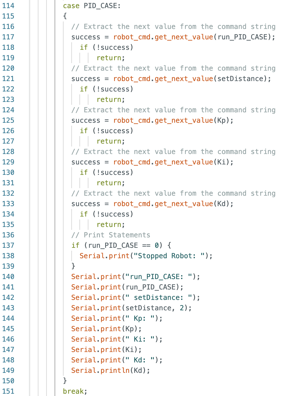
Below is the Jupyter Notebook Command and corresponding Arduino case to start/stop the PID controller. The run_PID_CASE, setDistance, Kp, Ki, and Kd values sent from Jupyter Notebook are printed in the Arduino serial monitor each time a command is sent. These values were initalized as global variables and will be used in the PID controller that is written in the main void loop(). If a command to stop the robot is sent from Jupyter Notebook "Stopped Robot: " will also be printed in the Arduino serial monitor.

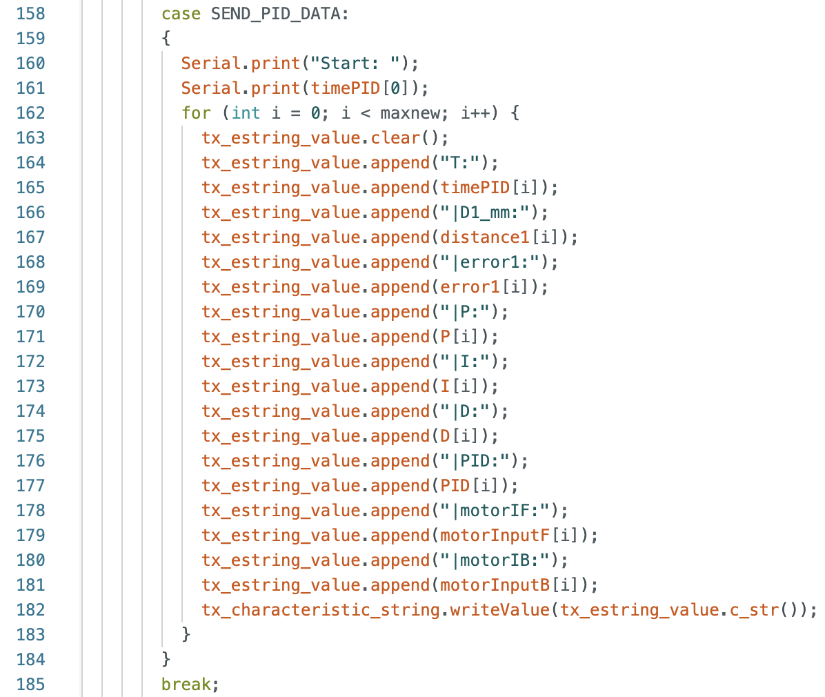
Below is the Jupyter Notebook Command and corresponding Arduino case to send the collected data. When data is sent the first time value is printed to the Arduino serial monitor to confirm that data was sent to Jupyter Notebook correctly. The time value is compared to the first time value in Jupyter Notebook.

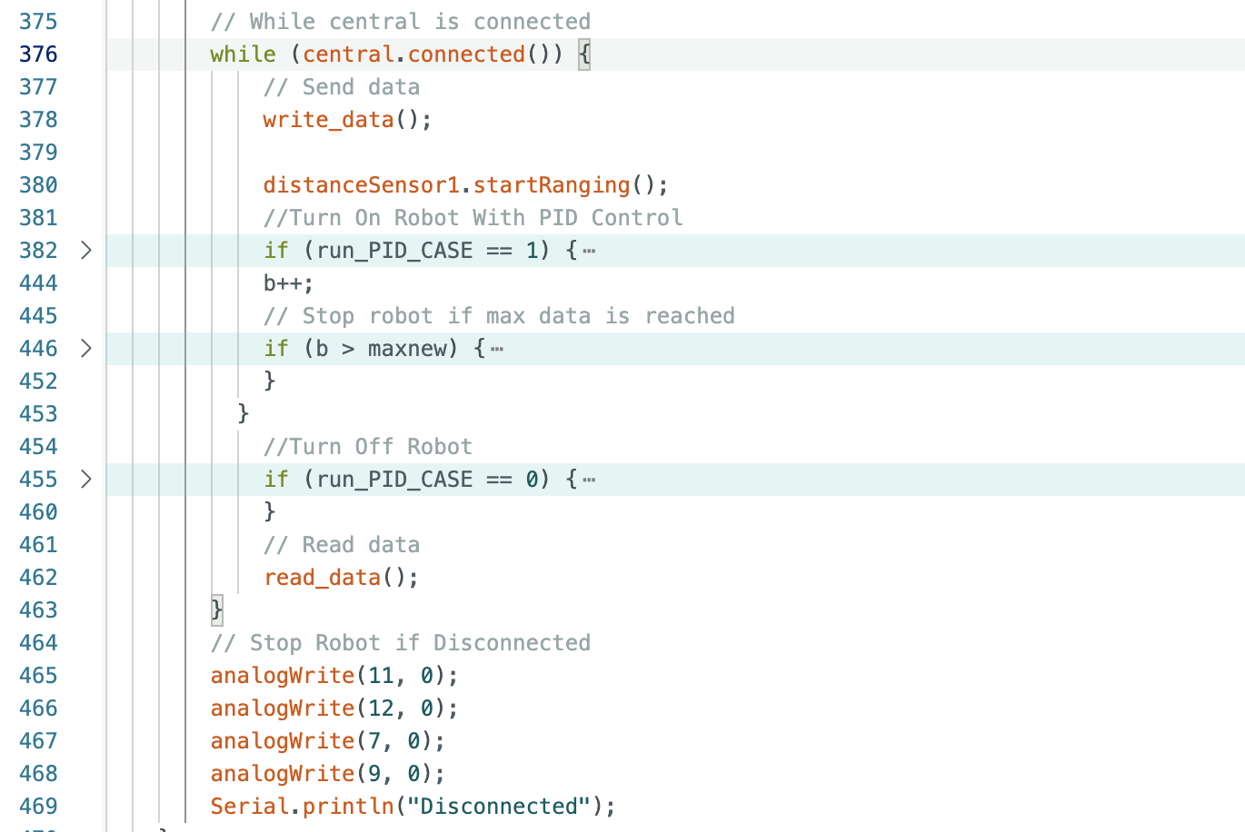
In addition, a hard stop was implemented on the Artemis to stop the robot if the Bluetooth connection fails. The pin output values are all set to zero outside of the while (central.connected()) loop. The code for this is inside the larger void loop() and is seen below (lines 465-469):
The above link has the full final version of the code used during the lab to collect distance measurements, extrapolate distance measurements, and move/stop the robot. I attached the link for my own reference in the future. The below steps show how and why I wrote each piece of the code.
For the position control task the robot drives as fast as possible towards a wall and stops when it is 1ft away from the wall. The ToF sensor on the front of the robot will be used to determine the distance the robot is from the wall. The implemented PID control is also shown to be robust to changing conditions including starting distance and floor surface.
For this task I choose to use the long distance mode for the ToF sensor as I was testing the robot for longer distances ranging from 6ft to 13ft and the range for the ToF sensor when using the long mode is 4m (13.12ft). The ToF sensor error can be at most 4000mm. To determine the sampling time of the ToF sensor I found the time between each new distance measurement by temporarily adding the lines below to the code that runs when the case to start the robot is called:

The sampling period was found to be 100ms, resulting in a sampling frequency of (1/0.1s) = 10Hz for distance measurements. To find how fast the PID control loop is running I printed the value for dt that is calculated each time the PID loop runs:

The PID loop runs at around 8ms (1/0.008s = 125Hz). The PID loop is running faster than the ToF sensor produces new distance readings. This will be explored later in the lab as the ToF sensor data will be extrapolated to use estimated data when there is no new ToF sensor distance measurement.
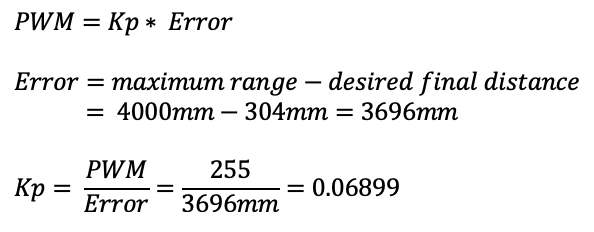
The first control input I worked on was the Kp input for proportional control. I estimated the value to be around 0.06899 by using the below equation to solve for the PWM values. I wanted to minimize overshoot, so to find the value for the error I subtracted the final desired distance from the maximum error based on the ToF sensor readings. The equations used can be found below:
The initial loop used to find the PID value is:
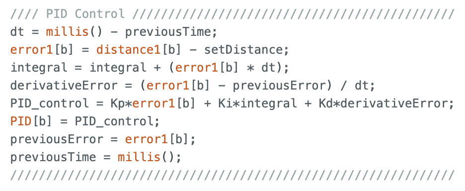
First the time difference (dt) is found and then the error is calculated based on the current distance and desired stopping distance. After the error is calculated the integral and derivative terms are solved for (both are 0 in this step). These PID equations were also used during the next step to find the Kd value for derivative control.
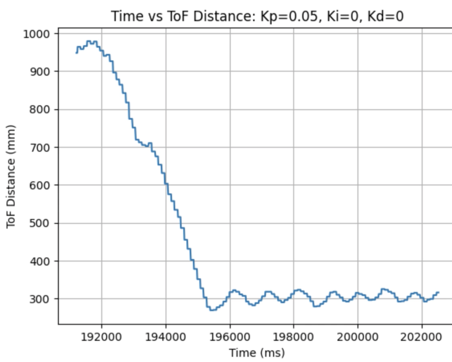
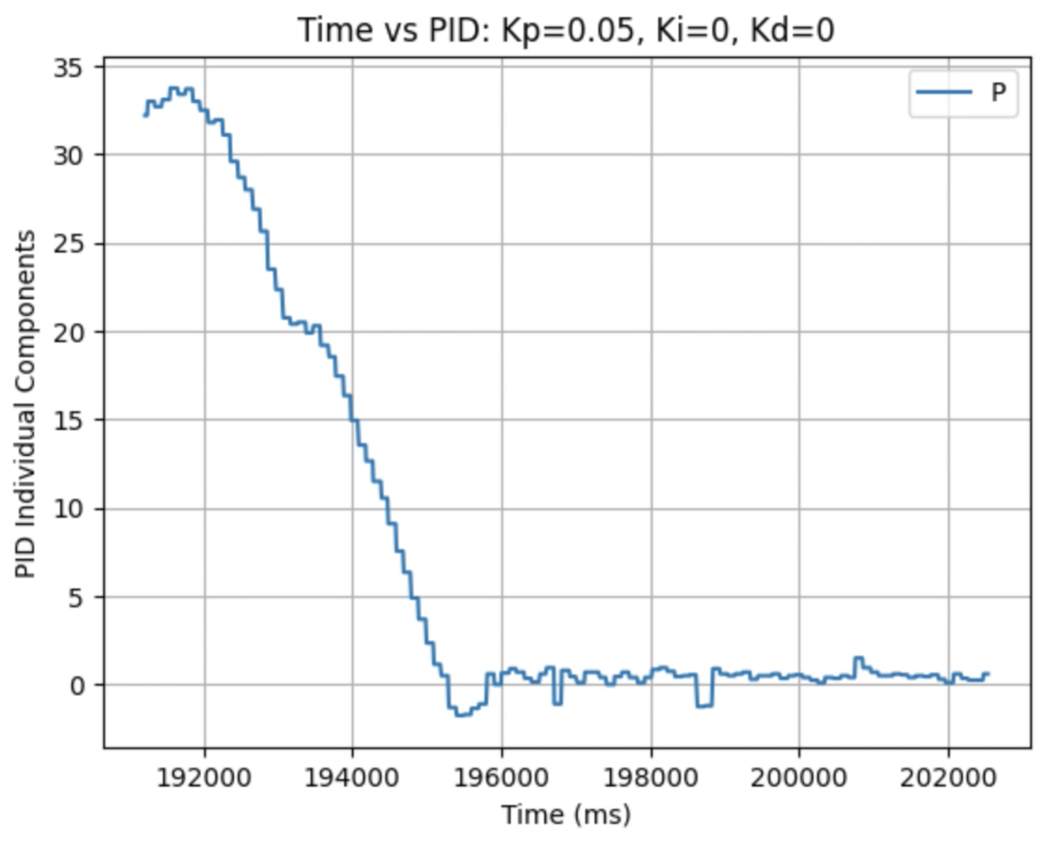
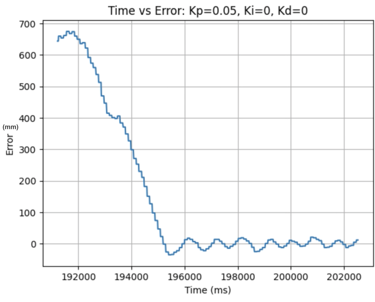
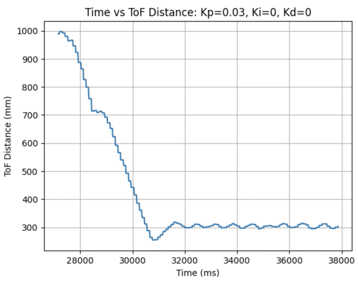
I used the calculated Kp value (0.06899) as an estimate. During the first physical testing of the system I tested a range of Kp values to determine at what point the robot oscillated around 1ft in front of the wall. Two of these Kp values are found graphed below. I determined that the Kp value should be set to 0.03 to minimize the error and oscillation present. The graphs showing Time vs ToF Distance, Time vs P Control, and Time vs Error for Kp = 0.05 and Kp = 0.03 can be found below:
Plots for Kp = 0.05:
Video for Kp = 0.05:
Plots for Kp = 0.03:
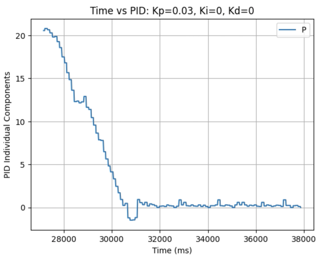
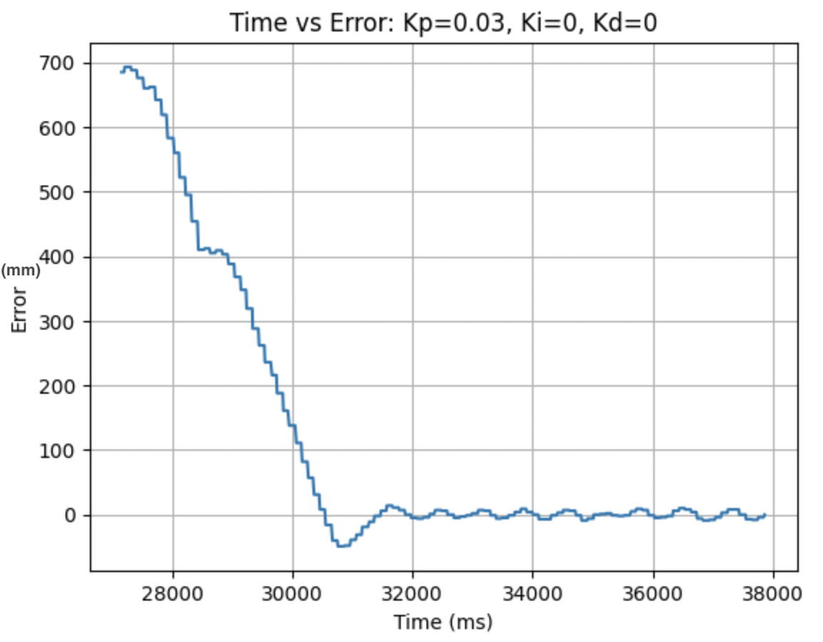
Video for Kp = 0.03:
In the above videos it can be seen that for a value of Kp = 0.05 the robot moves faster but overshoots and oscillates more, resulting in a greater error, compared to when Kp = 0.03. Larger Kp values resulted in the robot moving faster and having more error in the final position. Kp = 0.03 was the smallest value for Kp that resulted in the robot completing the full motion. For this first task I wanted to reduce oscillation, rather than achieve a faster speed and moved to the next step using Kp = 0.03. I focused on achieving a faster speed when tuning the integral Ki value, and prevented overshoot when tuning the derivative Kd value.
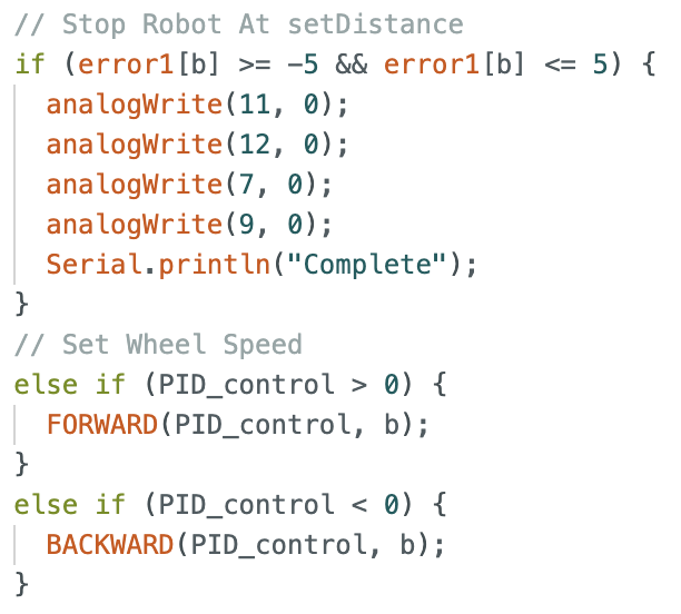
Stopping the Robot or Continuing Motion:
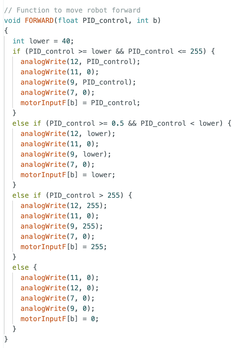
The robot is set to stop when the calculated error is less than 5mm. All pins are then set to zero. If the error is not within the stopping range than the function FORWARD is called if the PID value is greater than zero, or the function BACKWARD is called if the PID value is less than zero. The if statements and functions can be found below.
Stop when 1ft is reached or continue motion:
Forward motion:
Backward motion:
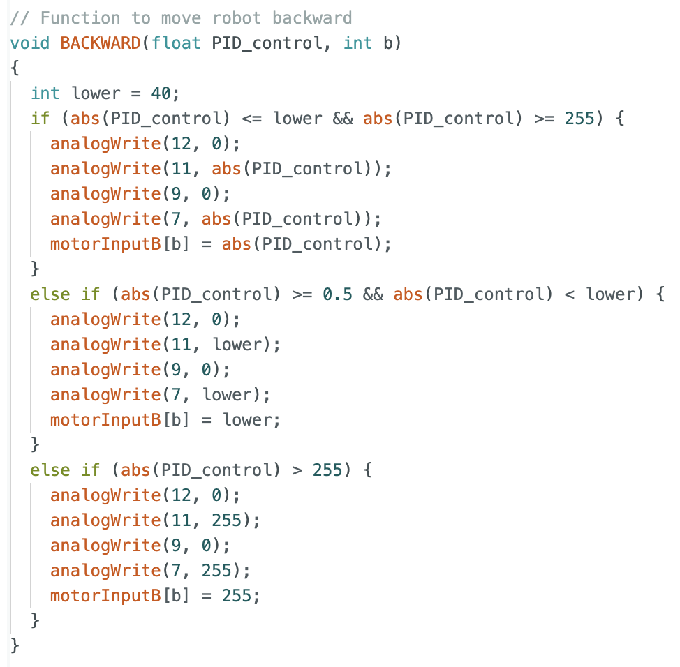
For PID values greater than or equal to 40 and less than or equal to 255, the PID value is used as the input PWM value for the motors. For values greater than 0.5 and less than 40 the input PWM value is set to be 40, because assigning values less than 40 would result in no motion of the robot. For values greater than 255, the PWM value is set to 255 as that is the maximum possible value for the motors.
Prior to writing the FORWARD and BACKWARD functions for scaling, I tried using map() to scale the PID values to PWM motor input values. The written code can be found in this folder This approach was not used because when running the robot, I repeatedly entered into a Fault Handler. In a first attempt to fix this problem I removed all code in the Arduino script that was not being used for this lab to reduce the size of the code, but that did not solve the Fault Handler issue. I then wrote the previously discussed functions to move the robot.
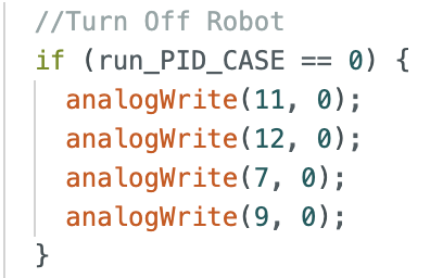
Another way to stop the robot are either intentionally stopping the robot by sending a "0" value for run_PID_CASE in Jupyter Notebook. Sending a "0" causes the following if statement in the while loop to set all pins to zero.
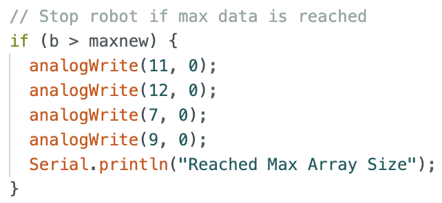
The final way that the robot stops is if the maximum value for the collected arrays is reached, causing all pins to be set to zero and stopping the robot. This is to ensure that each time the robot runs I know if the maximum array size is reached.
The next task I worked on was tuning the Kd value using proportional control and derivative control at the same time. I wanted to prevent overshoot and any oscillation of the robot. I increased the Kd value until the overshoot was reduced and the robot stopped at the 1ft desired distance from the wall. This Kd value was found to be Kd = 5. A video showing the robot at Kp = 0.03 and Kd = 5 is below:
Derivative Kick and Low Pass Filter:
For this task the ending setpoint distance does not change, resulting in the error derivative to be continuous. I did not need to implement anything to get rid of derivative kick because there is no changing setpoint. I did consult the reference provided in the lab instructions and read about derivative kick on this website, for future reference.
In addition a low pass filter for the derivative was not implemented as all of the calculated derivative error values were small.
For the next task I added the integral controller and inputed a Ki value. To start I set Kd to zero and tested a value of Ki = 0.00001 and Kp = 0.03. This resulted in the robot moving very fast into the wall. I then decided to decrease Ki until I found a value where the robot would stop in front of the wall, but for each value tested the robot ran into the wall. I then implemented wind up protection for the integral control to prevent the robot from overshooting and running into the wall. The Arduino code that was added can be found below:
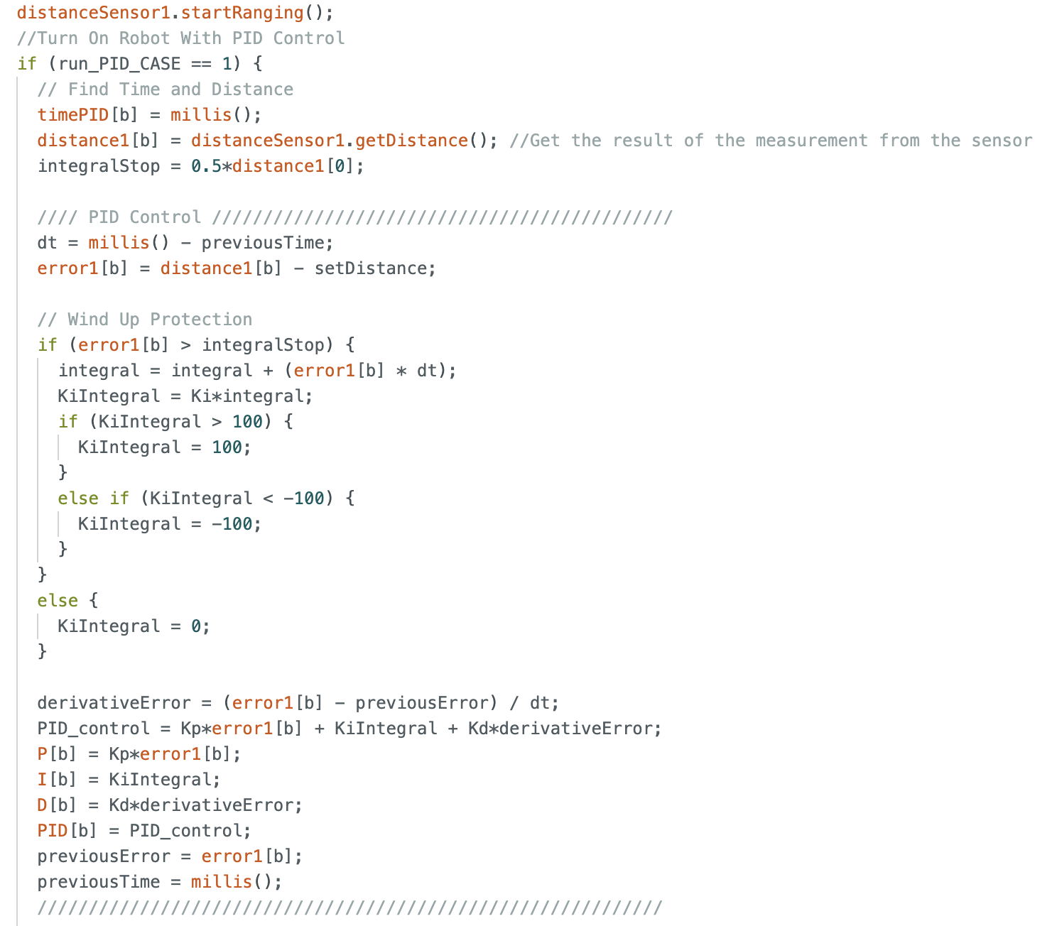
First a distance measurement is taken at the start of the robots motion to determine the total distance the robot needs to move and an integralStop value is set to be half of the total distance travelled. Each loop an if statement checks to see if the error is greater than the integralStop value. If the error is greater then integralStop a new integral value will be calculated. If the value of the integral term multiplied by the set Ki value is greater than 100 then there will be no further increase in the KiIntegral term used to find the PID control. In additon, if the error is smaller then the integralStop value then the new integral value will be set to zero. The integral term is the Ki value multiplied by the time integrated error. Without wind up protection the integral term will continuously increase causing the robot to not stop when the final distance is reached. Below is a video showing the KiIntegral (I) terms continuously increase until stopping at 100. The error term is not changing significantly, but the KiIntegral (I) term continuously increases.
After implementing wind up protection I found a Ki value that allows the robot to lightly run into the wall before pulling back. I started with a Kp value of 0.00001 which resulted in the robot driving too fast into the wall. I decreased this value until Ki = 0.000008 resulted in the following performance when Kp = 0.03 and Kd = 0:
Without wind up protection the robot accelerates quickly and the following behavior is observed:
I then added the Kd term found in the previous step. A value of Kd = 5 resulted in more overshoot than I wanted the robot to have. I increased the Kd value until the overshoot was again minimized. This resulted from a value of Kd = 8. For values above Kd = 8 there was no longer a noticable difference in minimizing overshoot. The behavior for Kp = 0.03, Ki = 0.000008, and Kd = 8 can be seen in the three trials below. The robot was started from a distance of 6.5ft.
The data collected from the last trial can be found below. I included the printed array of time, distance, PID values, and motor input to confirm that the data was collected properly.
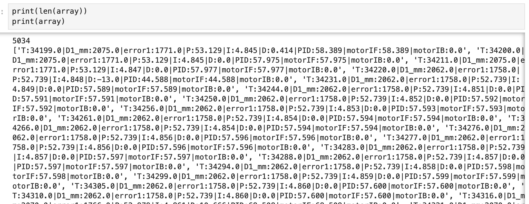
The three below graphs show the data for Time vs ToF Distance, Time vs Motor Input, and Time vs Error.
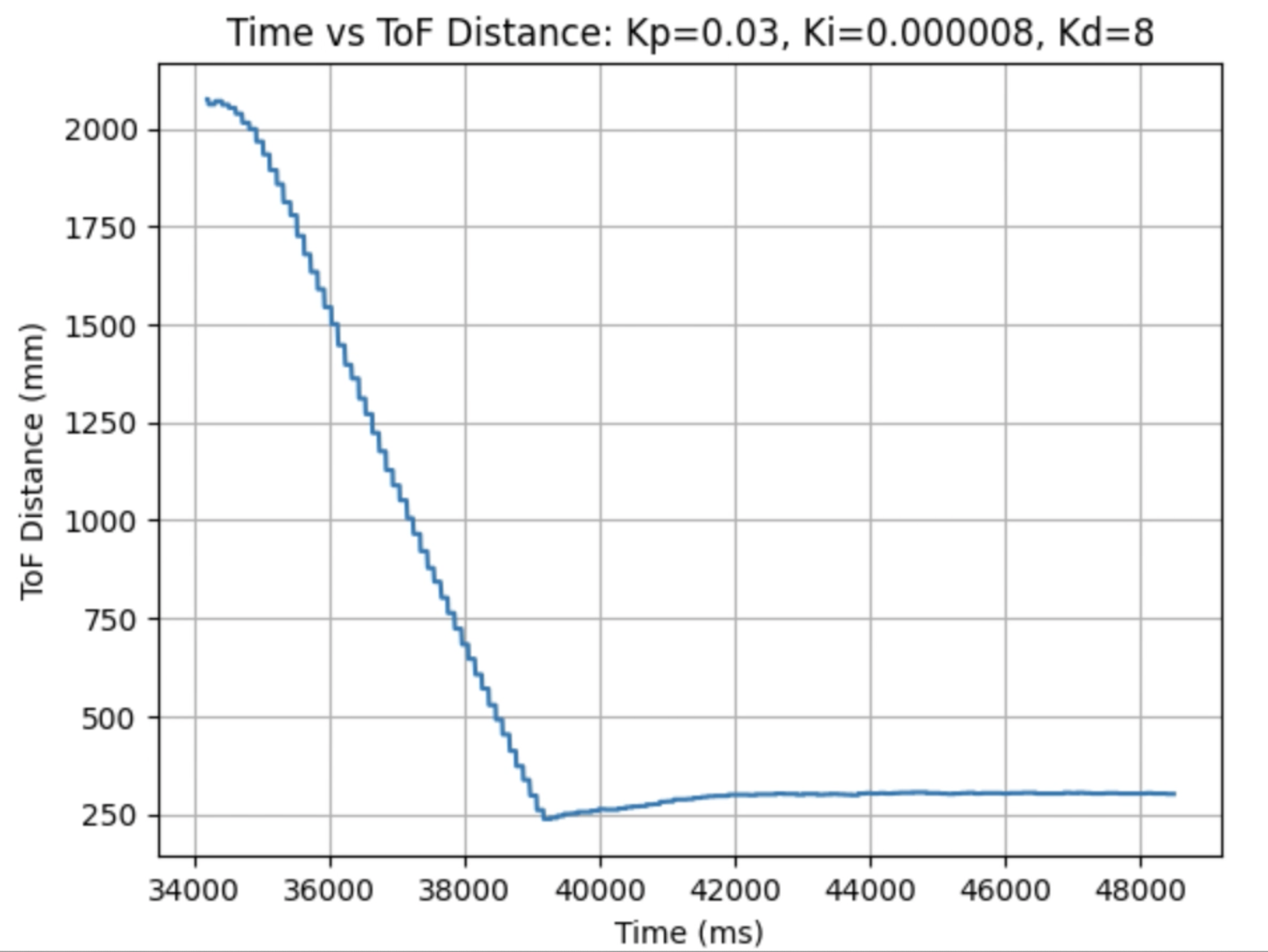
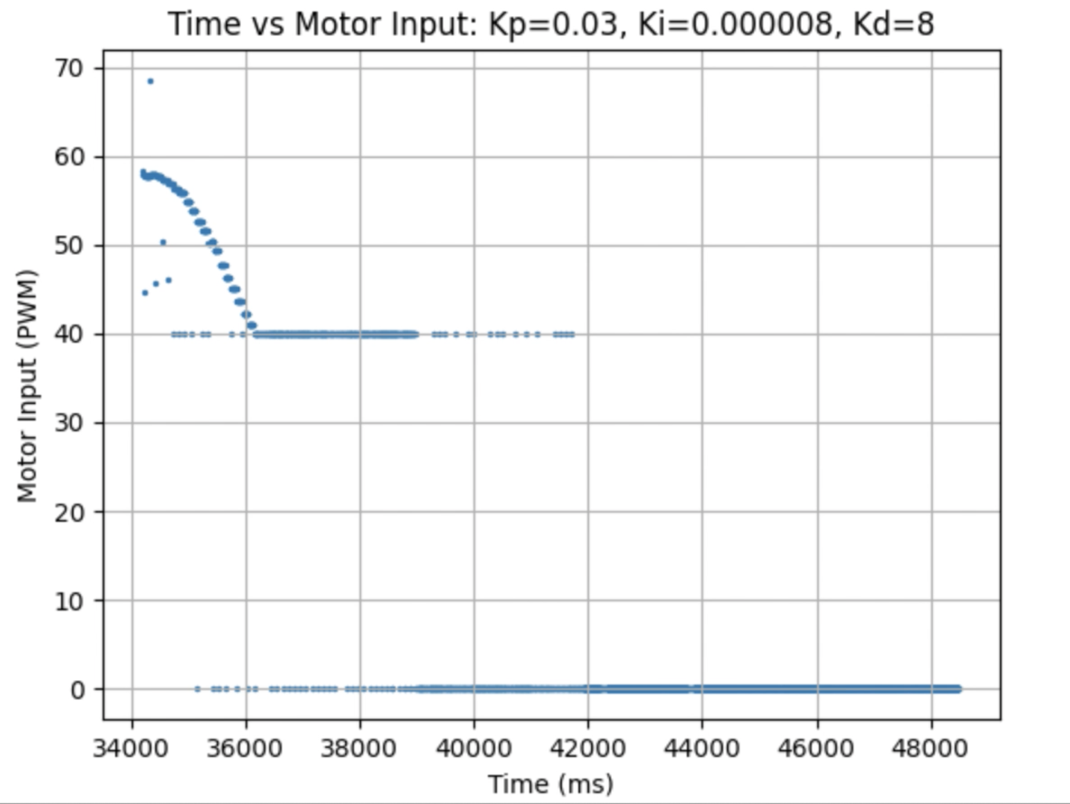
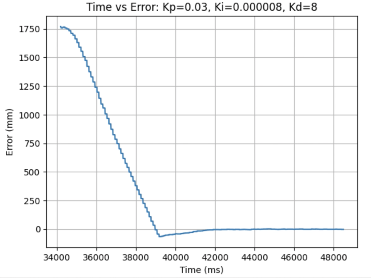
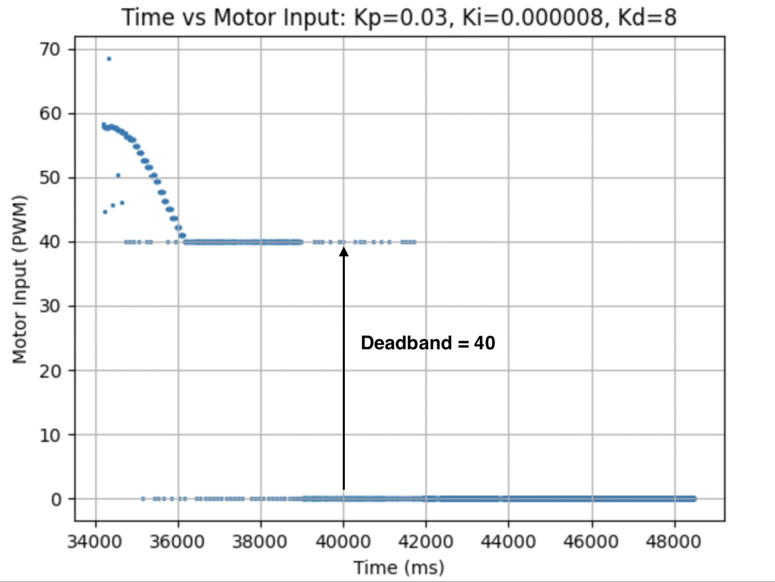
Graph Analysis and Deadband:
The above graphs for the distance and error reading show that there is minimal over shoot and the robot stops at the desired distance of 1ft away from the wall. The graph for Time vs Motor Input shows that the initial motor input is 58 and decreases until a motor input of 40 is reached. The deadband for the motors is 40. Any value between 0.5 and 40 (forward) or -0.5 and -40 (backward) will be set to 40 in order to produce a PWM value that causes the motors to move. I choose a lower bound of 0.5 and -0.5 to prevent the robot from overly moving after reaching the final distance. The functions used to produce forward and backward motion were discussed previously in the section for Proportional Control. When the robot stops the motor input changes to zero.
Maximum Linear Speed:
The maximum linear speed of the robot can be found using the Time vs ToF Distance graph. Using two points on the graph it can be found that (1506mm - 707mm)/(36105ms - 38258ms) = 0.37m/s
As stated previously in the lab in the Range and Sampling Time Discussion section, the sampling period was found to be 100ms, resulting in a sampling frequency of (1/0.1s) = 10Hz for distance measurements.
As stated previously in the lab in the Range and Sampling Time Discussion section, The PID loop runs at around 8ms, which is faster than the ToF sensor produces new distance readings. Extrapolation will be used to estimate the distance when new data is not available using past ToF distance readings.
Due to the ToF sensor running slower than the PID loop, extrapolation is used to estimate the distance using past data points. Below is the extrapolation equation:

This equation was implemented in the Arduino code. An if statement checks if the ToF distance sensor has a new distance reading. If the sensor has a new distance reading then that point is added to the distance_data array and the current time and distance are stored in time1 and dis1 variables. The previous time and distance from the last time there was a new distance measurement are stored in the time2 and dis2 variables. If there is no new distance reading the extrapolation equation is used as can be seen in line 395. The Arduino code for extrapolation is below:
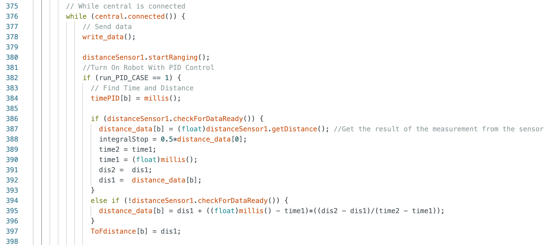
I outputted the raw data and extrapolated data to the serial monitor shown in the video below (units are mm). The first printed value is the raw data and the second printed value is the extrapolated data. The video shows that the extrapolated data readjusts whenever a new raw distance value is received.
Below is a graph for the raw and extrapolated distances. The graph is zoomed in to show that the extrapolated data (orange) readjusts to the raw data reading (blue) every time there is a new distance measurement. In the next section I ran tests using the extrapolated data.
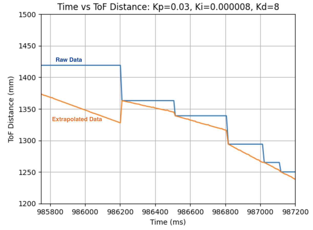
In addition, I tested the extrapolated distance PID control using different starting distances. The videos for each distance can be found below:
6.5 ft: Kp = 0.03, Ki = 0.000008, and Kd = 8
9.5 ft: Kp = 0.03, Ki = 0.000008, and Kd = 8
13 ft: Kp = 0.03, Ki = 0.000008, and Kd = 8
In the above videos it can be seen that the robot stops 1ft in front of the door, however for the largest tested distance of 13ft there were some runs where the robot did not go straight and instead curved towards the wall. This behavior can be seen in the second 13ft video. To correct this behavior orientation control can be implemented to keep the robot moving straight.
As a note, the PID control for the robot was tested on two different types of flooring as can be seen throughout the lab videos. The behavior of the robot on both surfaces was the same using the PID control. One surface was tile the other was laminate wood flooring.
See above: Completed in the 5000 Level Task: Integral Control (Ki) and Wind Up Protection Section.
Thank you to all of the TAs that answered my questions. I referenced the past lab reports of Liam Kain, Rafael Gottlieb, Larry Lu, Julian Prieto, and Ignacio Romo.
The objective of the lab is to control the car using open loop control, rather than the manual controller. Two dual motor drivers will be connected to the car's motors and the Artemis board. The dual motor drivers will be used to control the movement of the car.
The prelab involved reading about how to use an oscilloscope and determining how to connect the dual motor drivers to the motors and Artemis board. The lab materials include:
Below is a wiring diagram for the two dual motor drivers connected to the Artemis board, DC Motors, and 850mAh battery. The two VIN pins and the two GND pins on both dual motor drivers are connected together and then connected to the 850mAh battery. The GND pin of one of the dual motor drivers is connected to the GND of the Artemis board. There is a bridge between the BOUT1 and AOUT1 pins of the dual motor driver that is then connected to the DC motor. There is also a bridge between the BOUT2 and AOUT2 pins of the dual motor driver that is then connected to the DC motor. There is a bridge between the BIN1 and AIN1 pins on the dual motor driver and there is also a bridge between the BIN2 and AIN2 pins. On the dual motor driver that connects the drivers to the ground of the Artemis board (top dual motar driver in sketch below), the bridge between BIN1 and AIN1 is connected to pin 11, and the bridge between BIN2 and AIN2 is connected to pin 12. On the other dual motor driver (bottom dual motor driver in sketch below) the bridge between BIN1 and AIN1 is connected to pin 7, and the bridge between BIN2 and AIN2 is connected to pin 9. The pins used in this lab were chosen from the remaining pins on the Artemis board (after the previous lab). The parallel-couple of the two inputs and two outputs on each dual motor driver allows for twice the average current to be delivered without overheating.
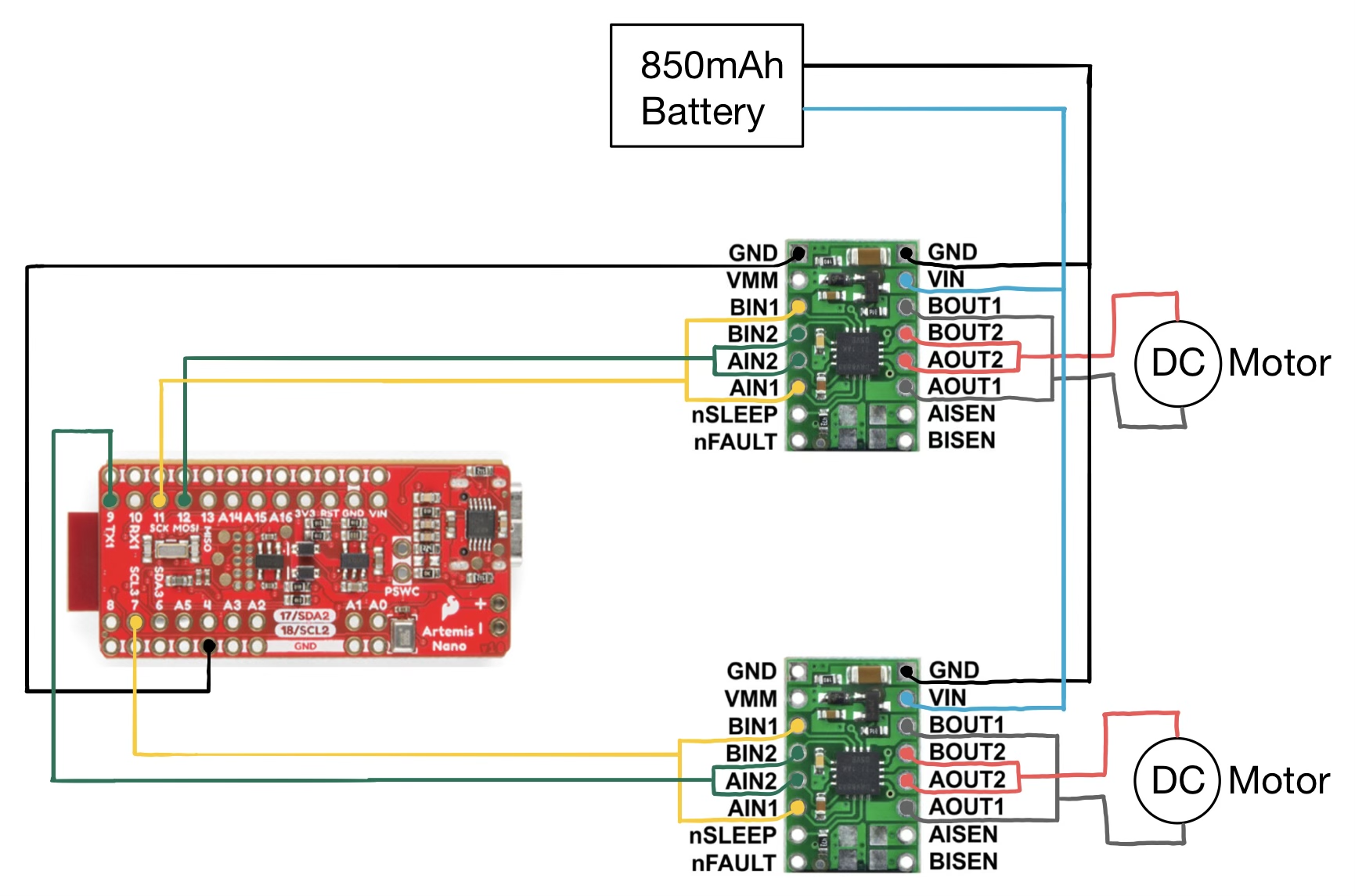
The Artemis board and the motor drivers/motors are powered from separate batteries. The Artemis board is powered using a 650mAh battery and the motors are powered using a 850mAh battery. Having the Artemis board and motors powered by different power sources avoids any potential transient effects and allows each component to function independently. Any potential current changes in the motors will not affect the Artemis board. In addition, the motors require a higher current battery, which is the reason the 850mAh battery is used to power the motors.
The below image is a picture of the power supply and oscilloscope connections. The positive power supply wire (red, towards the top of the picture) is connected to the positive wire of the battery. The ground wire of the power supply (black) and oscilloscope (black) is connected to the same ground wire of the battery (near the middle of the picture). The input for the oscilloscope (near the bottom of the picture) is connected to the wire that will be attached to one of the motors. Each of the four wires that will be attached to the motors was tested to determine if the circuit was assembled correctly and a PWM signal was shown on the oscilloscope.
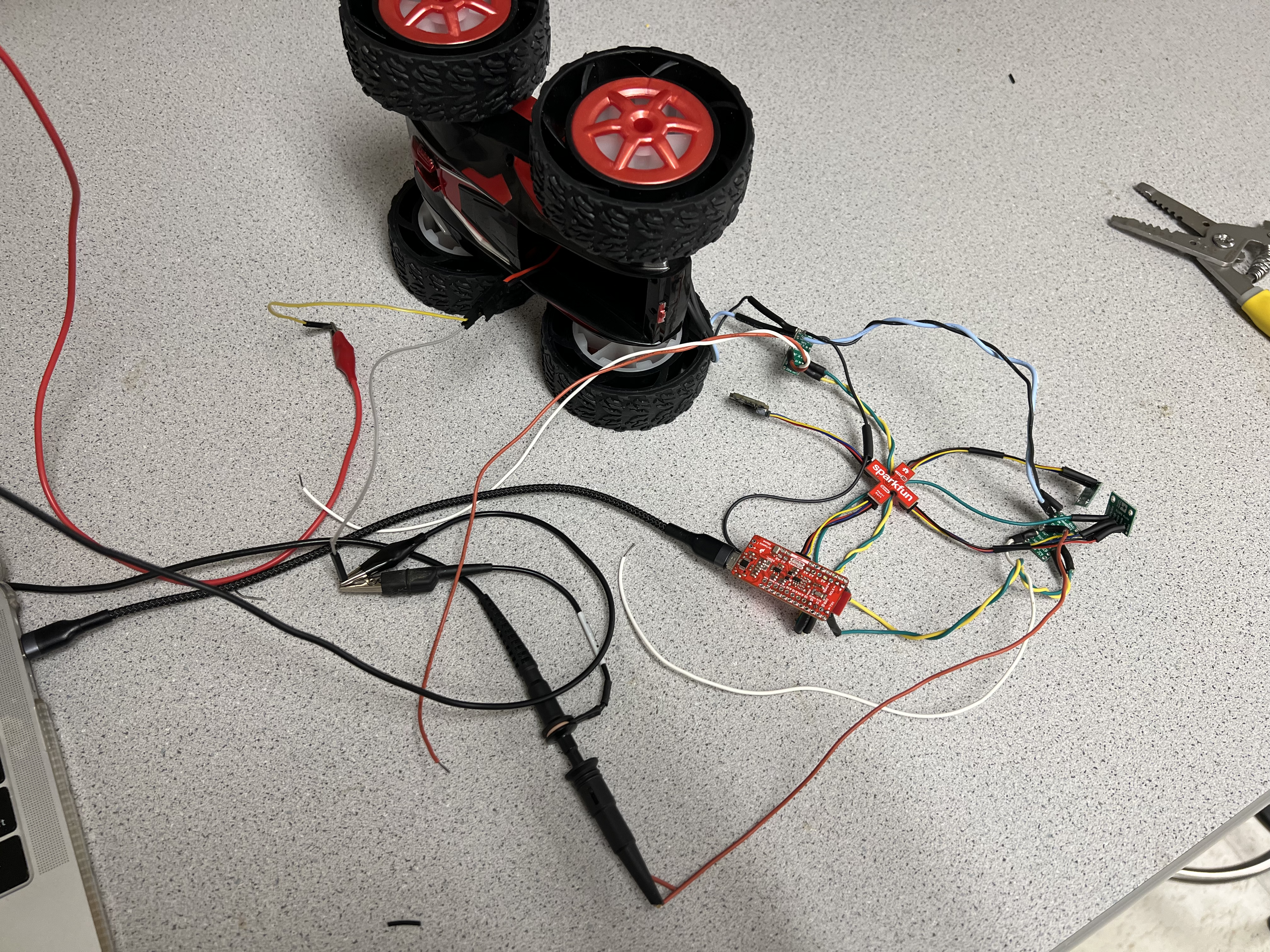
Picture of oscilloscope (left) and power supply (right) connected to the circuit:
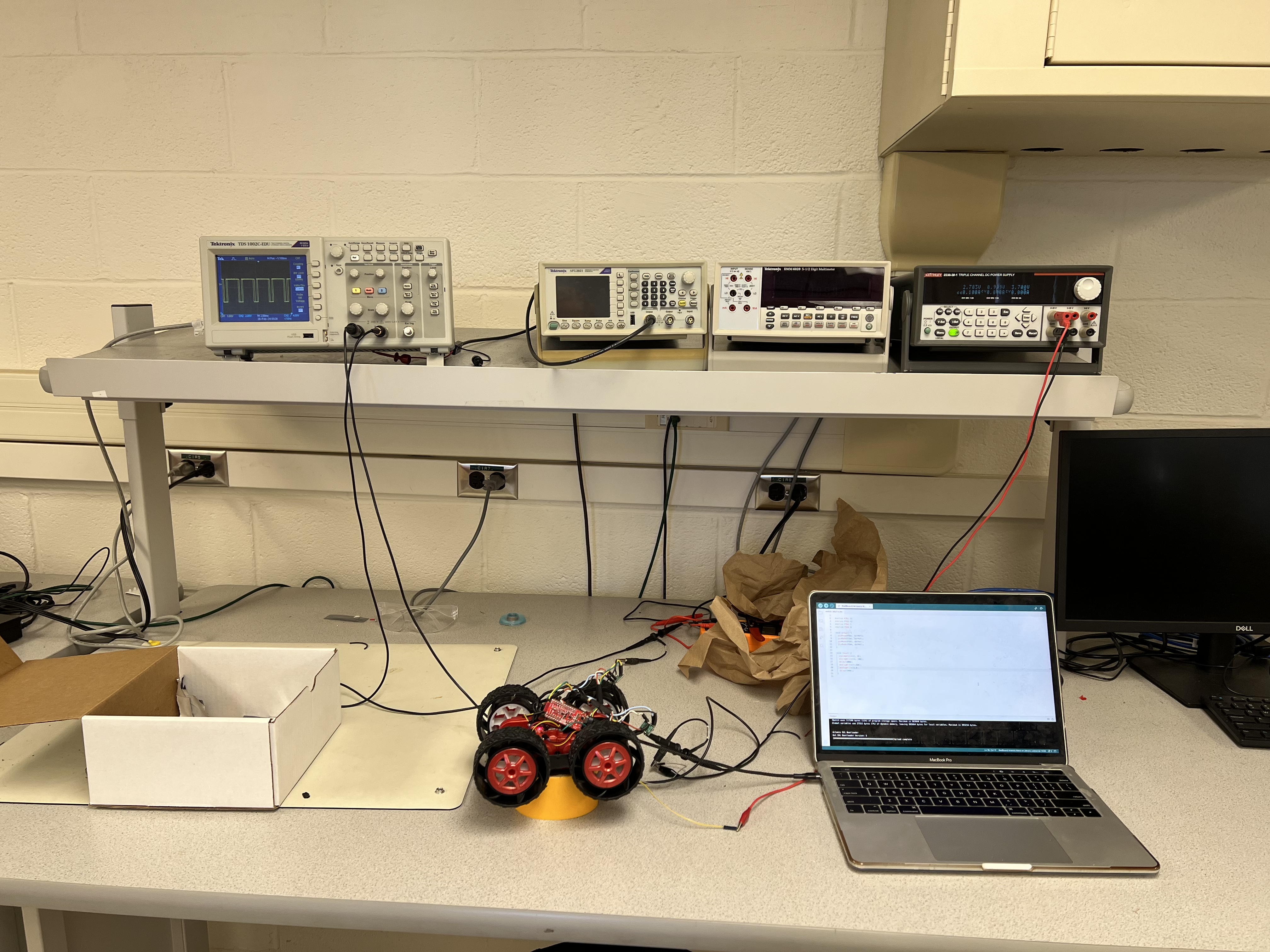
The voltage of the 850mAh battery is 3.7V. In place of using the battery, a power supply was used. The output of the power supply was set to 3.7V to represent the battery power that will be used later on during the lab. Each pin was tested independently of each other. In the Arduino IDE code, one pin was set to have an output of 200, while the other pins all had an output of 0. This was repeated for all four pins. The positive output voltage to the motor was displayed on the oscilloscope and indicated a constant voltage output at each time. The PWM values show that power can be regulated on the motor driver output.
Channel 3 of the power supply was used. 3.7V was used to test the motor driver circuit.
Picture of the oscilloscope output:
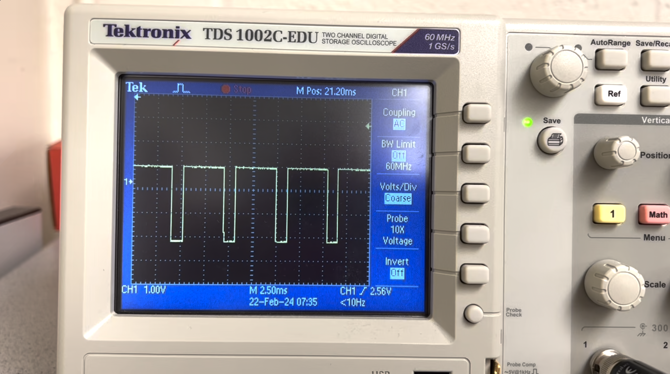
The below four videos show the output for each pin that was tested:
Pin 11, Output 200:
Pin 12, Output 200:
Pin 7, Output 200:
Pin 9, Output 200:
The below Arduino code shows how each of the wires to the motors were tested. Pins 7, 9, 11, and 12 were defined and analogWrite() was used to assign each pin number the tested output value. In the below example pin 11 is set to have an output of 200, and all of the other pins have an output of 0.
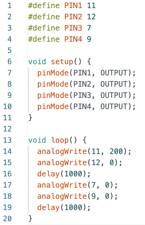
The wheels on each side of the robot were tested individually at two different output values. The power supply used at the beginning of the lab (3.7V) was used to power the motors. Pins 7, 9, 11, and 12 were tested at output values of 50 and 200. While testing each side of the robot I observed the direction and speed that each wheel turned. The wheels rotated faster for the higher output at 200 compared to the output at 50. For the higher output value of 200, the wheels reached the final set speed faster compared to the lower set speed. When rotating at 50 the wheels took longer to start rotating. From the perspective of the videos pin 7 rotates counter clockwise and pin 9 rotates clockwise. Pin 7 and pin 9 move the wheels on the same side of the robot in different directions. In addition, from the perspective of the videos pin 11 moves clockwise and pin 12 moves counter clockwise. Pin 11 and pin 12 move the wheels on the same side of the robot in different directions. To consolidate the report, all of the videos taken can be found in this folder: Folder Link Below are videos of pin 12 and pin 9 with an output value of 200.
Pin 12 with an output of 200:
Pin 9 with an output of 200:
The Arduino code to test the wheels is found below. One pin was set to have an output value of either 50 or 200 and all other pins were set to have an output value of 0. This is the same code that was used in the previous section to test if the circuit was working properly before sautering to the motors.
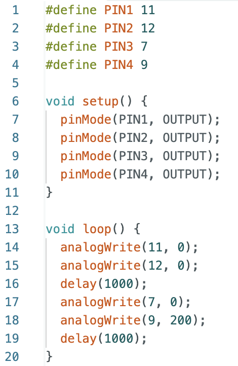
After testing each side of the robot, all of the wheels were tested at the same time. The 850mAh battery was used to power the motors instead of the power supply. The below video shows both sides rotating while the motors and Artemis board are both connected to their respective batteries.
The Arduino code to test the wheels on both sides of the robot is found below. Pins 9 and 12 were set to have an output of 200 and pins 7 and 11 were set to have an output value of 0. This is the same code that was used in the previous section to test both sides of the robot individually.
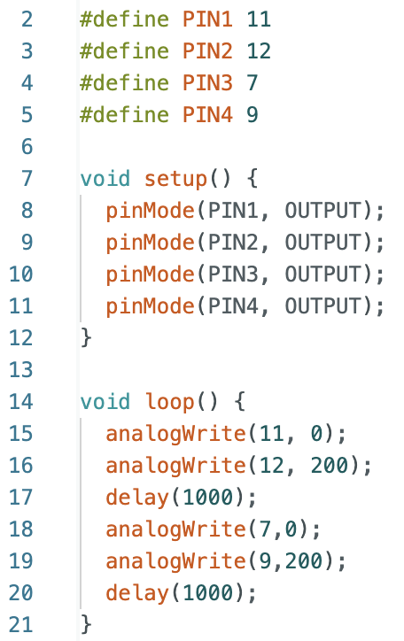
Below is a labeled picture showing all components on the robot. Including the 650mAh battery, Artemis board, IMU, two ToF sensors, two motor drivers, and a breakout board. The 850mAh battery to power the motors is on the other side of the robot.
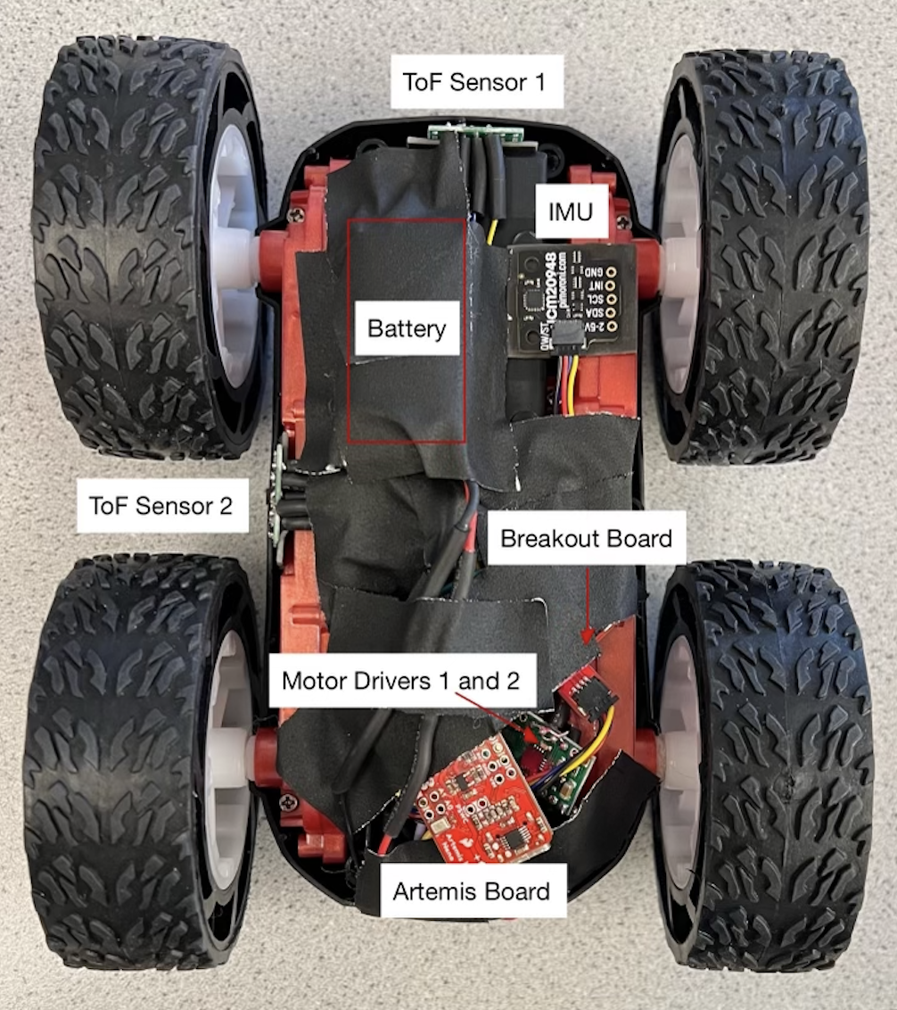
After connecting all components to the car I decided to test how the robot moves. The video below shows my first test for having the robot drive on the ground. In the video, the robot initially moves towards the left when the pins used for the motors have the same output value. This trend was noticed in future steps of the lab when determining how to calibrate each of the motors.
The below code shows the loop used to run the robot on the ground.

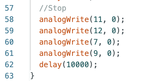
Below is a diagram of the entire wiring that is used on the robot:
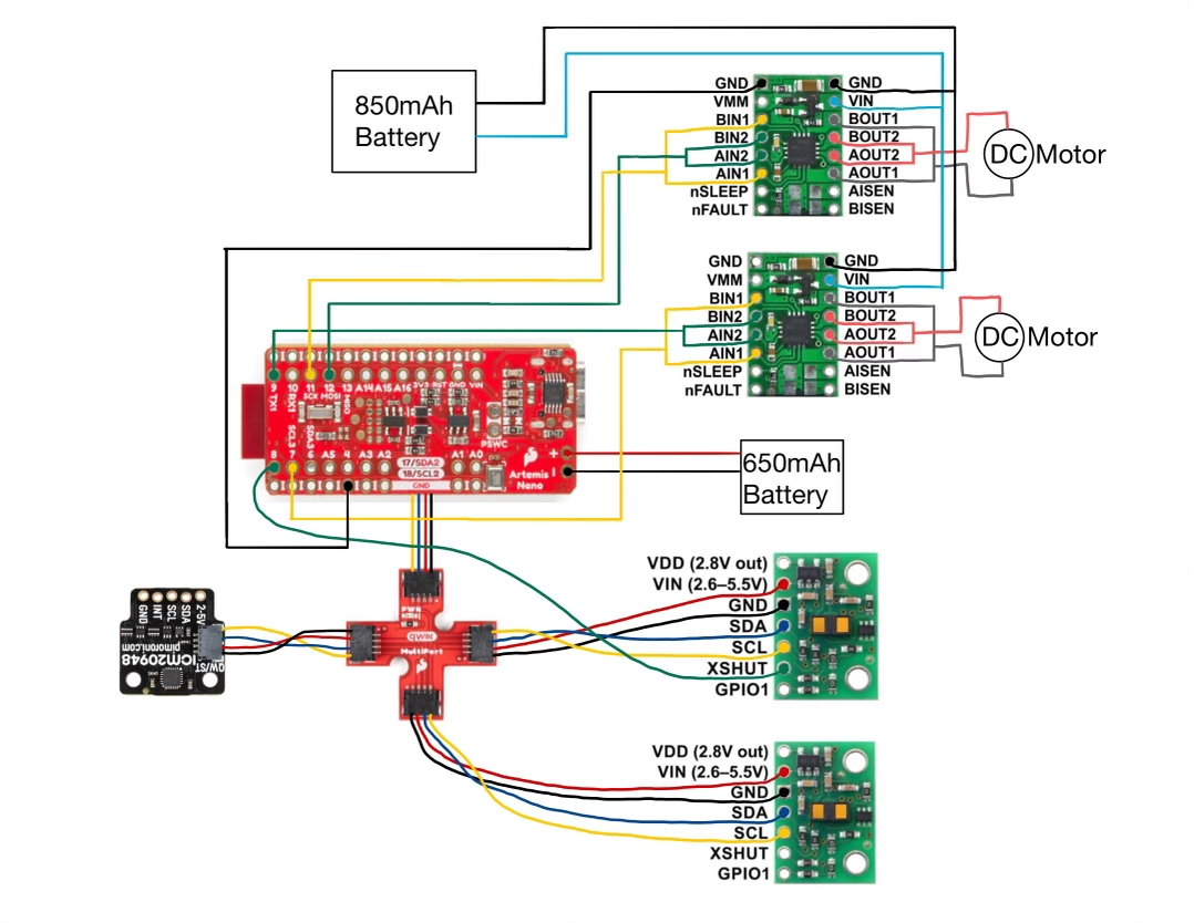
During this step of the lab, I used Bluetooth to send a command from Jupyter Notebook to run different output values more easily compared to uploading Arduino IDE code every time I wanted to change the output value of a pin. The below images show the Jupyter Notebook Command and the Arduino IDE case that uses analogWrite() to move the robot.

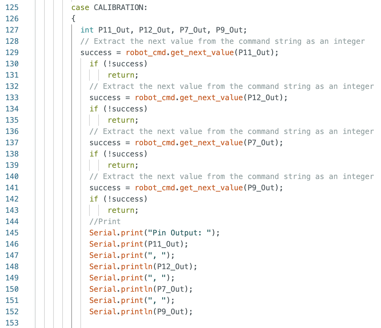
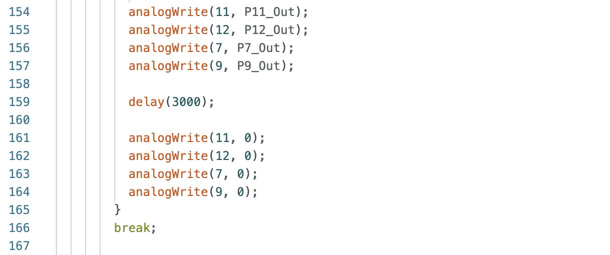
The lower limit PWM value is the lowest output value that a pin can be set to that will still result in continuous motion of the robot. The wheels on one side of the robot were tested, while the wheels on the other side remained stationary. The lower limit PWM for pin 11 (right side) was found to be 59. The lower limit PWM for pin 7 (left side) was found to be 50.
Pin 11 (Right Wheels) with an output of 59:
Pin 7 (Left Wheels) with an output of 50:
I also found the PWM value for both wheels when they are being used together, starting when the robot is stationary. The output value was found to be 35 for both wheel sides. The video showing the robot moving when both wheels (pins 11 and 7) have an output value of 35.
Note: During lab office hours I asked a TA (Larry Lu) about how the surface conditions affect the PWM values. Specifically I asked if testing the robot on the floors in my apartment (laminate wood flooring) would change the lower limit PWM value compared to the tile floors in the lab and hallways. I tested the robot's lower limit PWM value at my apartment and received the same PWM values. The PWM values may start to differ if the robot is travelling over a surface with a lot of friction such as a carpet or outside in the grass. This information is helpful to know as I can better understand the operating conditions of the robot.
The wheels of the robot do not spin at the same rate and a calibration factor needed to be implemented. The below video shows the robot moving in a straight line, starting at 7 feet and then continuing past the end of the tape measure. For the demonstration, pin 11 was set to an output of 60 and pin 7 was set to an output of 70. In addition to the below video, the robot was run multiple times at varying input values. My first tested value was pin 11 at an output of 60, which is close to the found PWM value from the previous step. When pin 7 was set to an output of 51, the robot continuously moved towards the left. Through trial and error I found that an output of 70 for pin 7 kept the robot moving in a straight line. I used these found values for reference during future tests: 70/60=1.166666666666667.
I increased the output of pin 11 by 20 for each test and multiplied the value for pin 7 by 1.166666666666667. This incrementation worked for all tested pin 11 and pin 7 values until I reached an output value of 220 for pin 11. The calculated output value for pin 7 should be 257, rounded down to 255 due to 255 being the maximum output value. For this test the robot continuously moved towards the right and the value for pin 7 needed to be lowered to 250 to keep the robot moving straight. Due to this discovery, I decided to also test an output value of 210 for pin 11, the calculated output value for pin 7 should be 245. In order to keep the robot moving straight, and not to the right I needed to reduce the output of pin 7 to 240. The trend shows that after an output of 200 for pin 11 the calibration factor to find the corresponding output value for pin 7 starts to differ.
In addition, as a final test I wanted to determine how low I could set the output values while still having the robot move in a straight line for at least 6 feet. I set the output value of pin 11 to 40 and calculated the output value of pin 7 to be 47. For these output values, the robot moved in a straight line for more than 6 feet. When I set the output value for pin 11 to be lower than 40 the wheels began to stall and hesitate before rotating compared to the other side of the robot. I also included a video at the end of the section showing the wheels spinning.
To produce the robots motion the same Arduino IDE case and Jupyter Notebook command were used from the previous section. The length of the delay was changed depending on how fast the robot moved (to prevent the robot from running into a wall). All of the recorded videos are in this folder.
Below is a graph showing all of the tested values as data points. In addition, I plotted the trendline for all data points, as well as the trendline for all of the data points except for the last two that began to differ from the previous measurements. The slope and y-intercept were also found for each trendline. The calculated slope is the calibration factor. The slope excluding the last two data points, 1.165 is close to the 1.166666666666667 value.
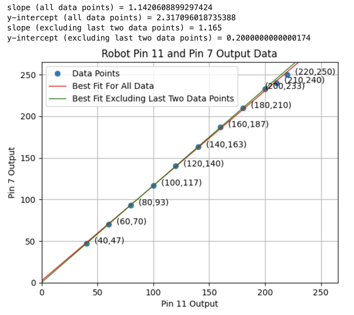
Video showing wheels hesitating when pin 11 (right) has an output of 35 and pin 7 (left) has an output of 41:
I also tested the calibration factor when the robot is going in "reverse" (with the robot moving in the direction away from the ToF sensor on one end). I initially tested the previously found output values with the corresponding pins on each wheel side, with pin 12 having an output of 60 and pin 9 having an output of 70. I found that by doing this the robot moved towards the left. I decided to switch the output values; pin 12 has an output of 70 and pin 9 has an output of 60). The robot moves straight using these output values. I find this interesting as it confirm my previous thoughts about one side of the wheels being slightly misaligned.
Below is a video showing open loop control of the robot. In the video the robot moves forward, turn towards the right, moves backward, stops, spins counterclockwise, stops, spins clockwise, and then stops. I used output values found from the calibration graph.
Arduino code for robot motion:
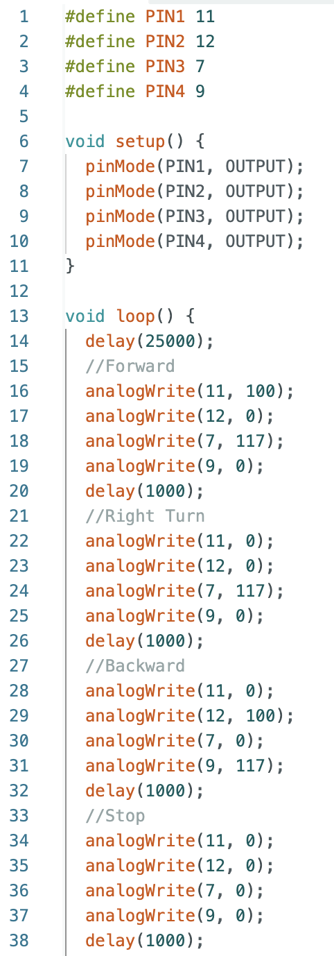
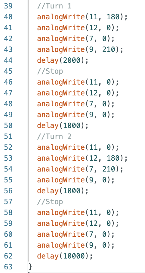
Below is the image of the oscilloscope when connected to the circuit. The wheel motors are powered using the battery. During lab office hours I asked a TA why the oscilloscope outputs were more noisy compared to the oscilloscope outputs from earlier in the lab and it is most likely because the circuit is now connected to the motors that result in more noise compared to when the circuit was not connected to the motors on the robot.
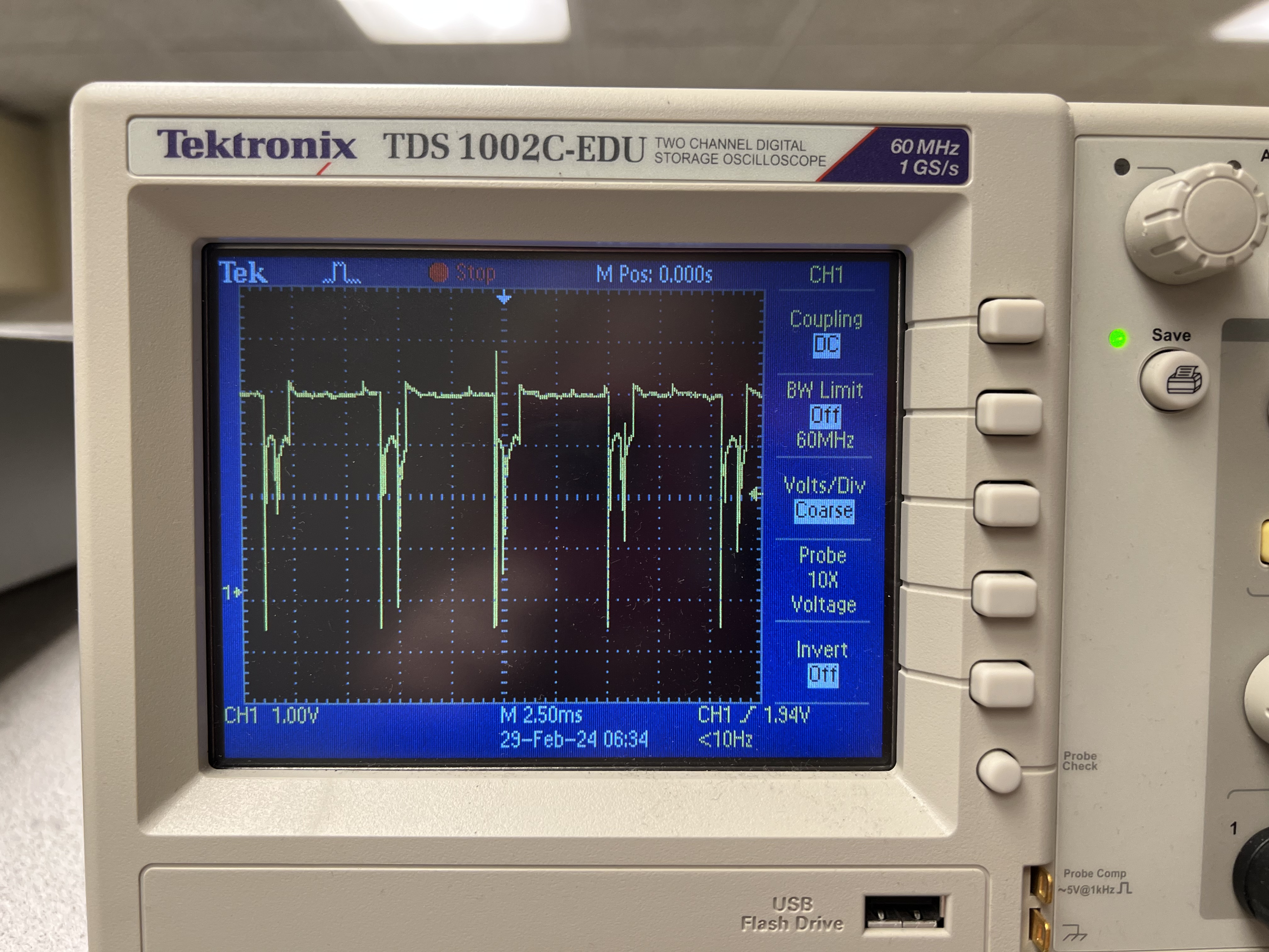
From the image its can be seen that one horizontal block along the x-axis is 2.50ms and one vertical block along the y-axis is 1.0V. The period of the PWM signal is about 2.6 horizontal blocks, which is equivalent to 6.50ms (0.0065s). The frequency analogWrite() generates is about 1/0.0065s ~= 154Hz. In lab 3 the sampling period of the ToF sensors was found to be 0.04s and the sampling frequency was 25Hz. The frequency analogWrite() generates is fast enough for the motors on the robot when running tests as well as when using data from the ToF sensors. Manually configuring the timers to generate a faster PWM signal will allow for more control over the movements of the robot and a more steady PWM signal.
The code used during the oscilloscope observation is below:
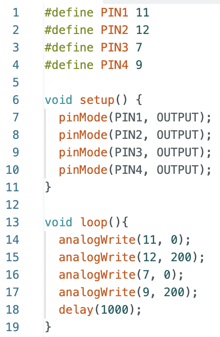
The lowest PWM value for each side of the robot was found by running the robot with an initial output of 60 for pin 11 and 70 for pin 7 to correspond with the found calibration values. The robot ran with these outputs for 3 seconds and then all pin outputs were set to zero expect either pin 11 or pin 7. Either pin 11 or pin 7 remained turned on for another 3 seconds, but decreased to a lower output value. I ran the robot multiple times to determine at what output value the robot no longer moved. It was determined that for pin 11 the lowest PWM output is 35 and for pin 7 the lowest PWM output is 33. The videos for each pin can be found below.
Pin 11 with a lowest PWM value of 35:
Pin 7 with a lowest PWM value of 33:
In addition, the lowest combined wheel PWM value was found when both wheels were being used at the same time. The output value for both wheels (pin 11 and pin 7) is 25 when the robot is already moving. The robot was initially run with an initial output of 60 for pin 11 and 70 for pin 7 for 1.5 seconds and then both wheels decreased to an output of 25 for 5 seconds. Below are two videos. One video shows the final output at 25 (the robot moves until the total set time of 5 seconds is over). The other video shows the robot stop before the 5 seconds is over and the motors stall when set to an output of 24, confirming the lower limit PWM value of 25 to keep the robot moving.
Both Wheels: Lower Limit PWM of 25:
Both Wheels: Tested value of 24:
The command line in Jupyter Notebook and the Arduino IDE case can be found below:

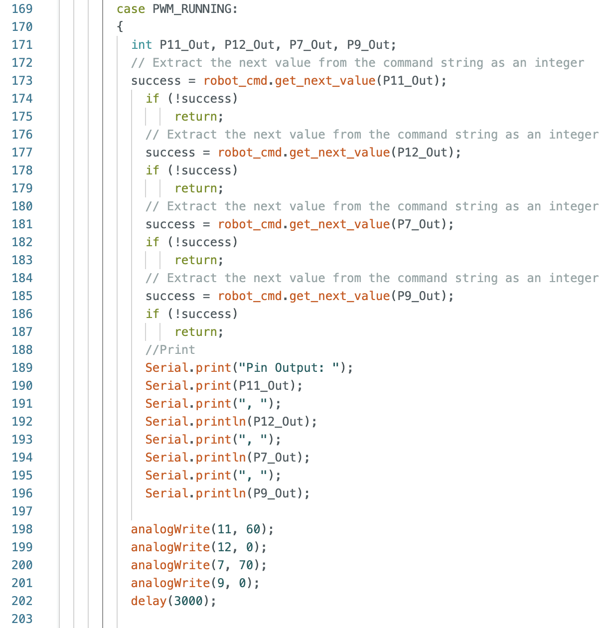
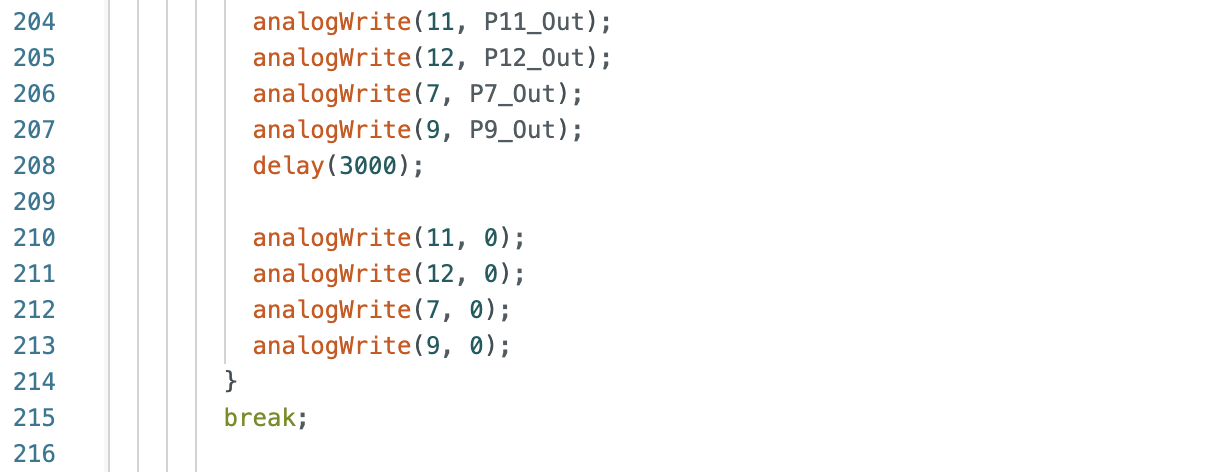
Thank you to all of the TAs that answered my questions. I referenced the past lab reports of Liam Kain, Rafael Gottlieb, Larry Lu, Julian Prieto, and Ignacio Romo.
The objective of the lab is to connect the time of flight (TOF) sensors to the Artemis board.
The prelab involved reading about the ToF sensor used in the lab. The lab materials include:
From the datasheet it was found that the I2C sensor address for the ToF sensor is 0x52. The two ToF sensors have the same address and one of the addresses will need to be changed in order to receive data from both sensors at the same time.
To use two ToF sensors, the XSHUT pin will be used to connect one of the ToF sensors to pin 8 on the Artemis board. The XSHUT pin will be set to LOW and then the I2C sensor address will be changed for the other ToF sensor that is on. After the I2C address has been changed the XSHUT pin will be set to HIGH, turning the other TOF sensor back on. This will allow for both ToF sensors to be used in parallel.
The placement of the two ToF sensors on the robot will impact the field of vision. Two long QWIIC connectors will be used to attach the ToF sensors. Longer connectors will allow me to position the ToF sensors in more potential ways compared to shorter wires. The potential arrangements of the sensors include (1) a sensor on the front and left side, (2) a sensor on the front and right side, (3) two sensors positioned on either side of the front of the robot, and (4) a sensor on the front and the back. Depending on the task at hand any of these sensor positions may be effective. If there is no sensor on the back of the robot there might be an issue if the robot needs to back up or move in reverse. If there is no sensor on the side then the robot might miss an obstacle that is located in a blind spot.
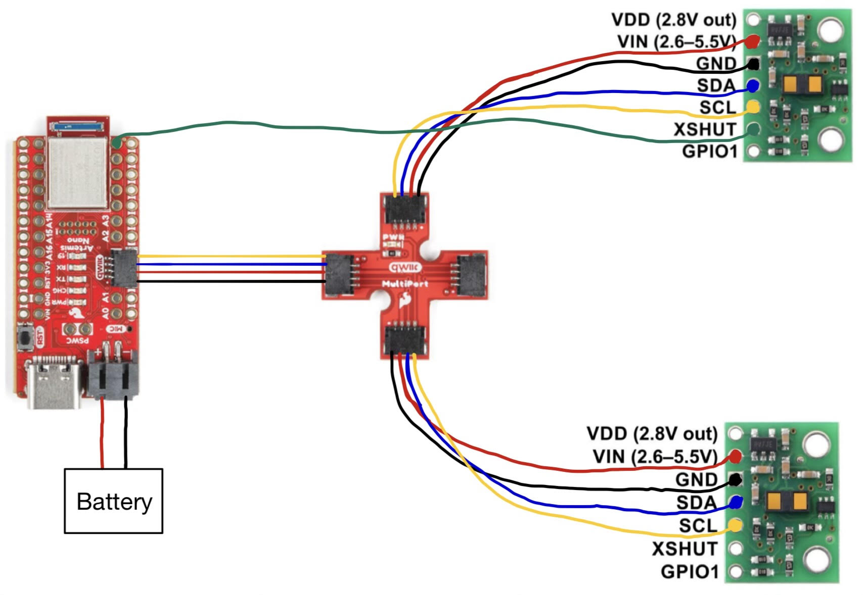
The Artemis board was powered using a battery:
ToF sensors connected to the QWIIC breakout board:
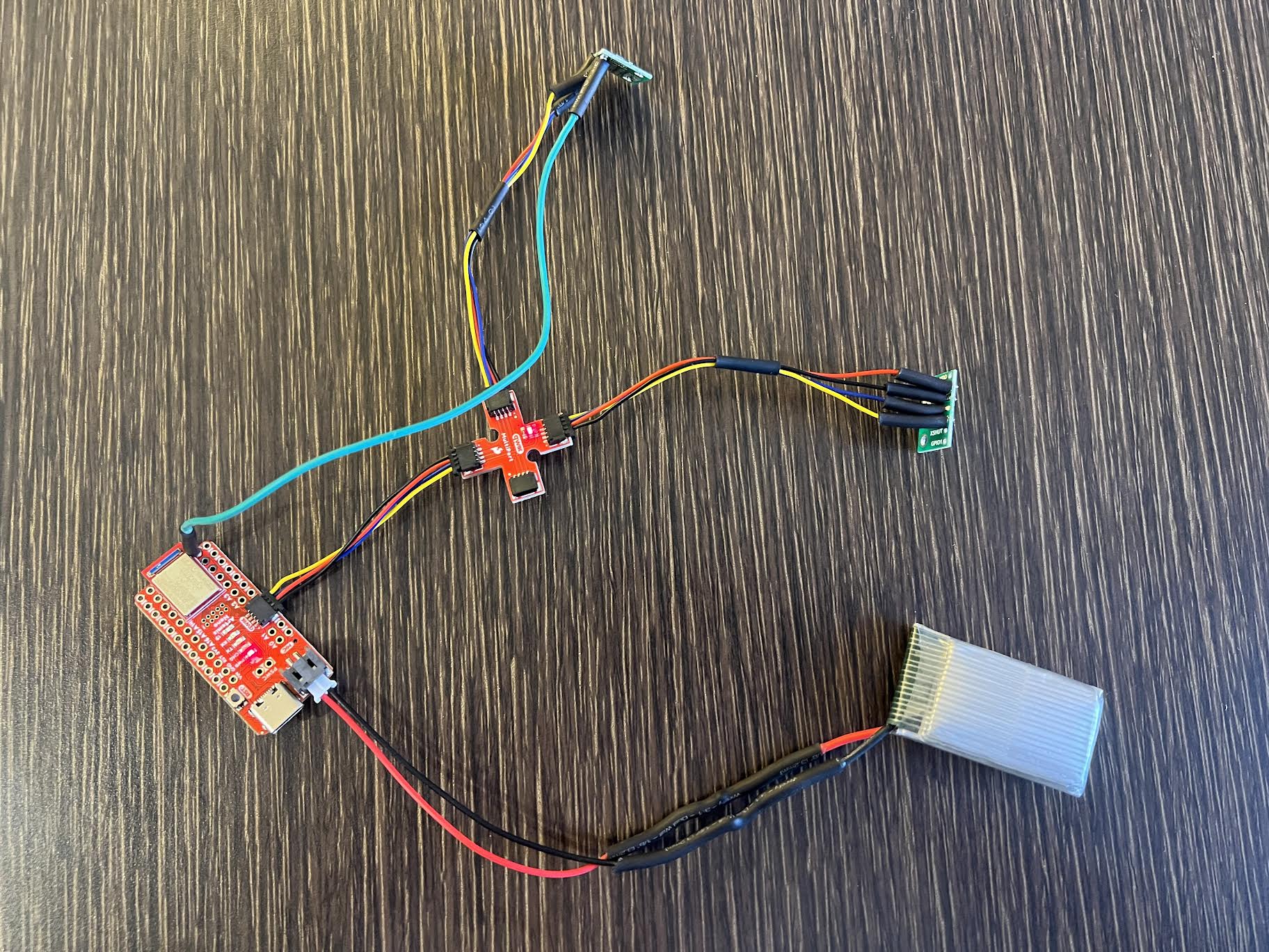
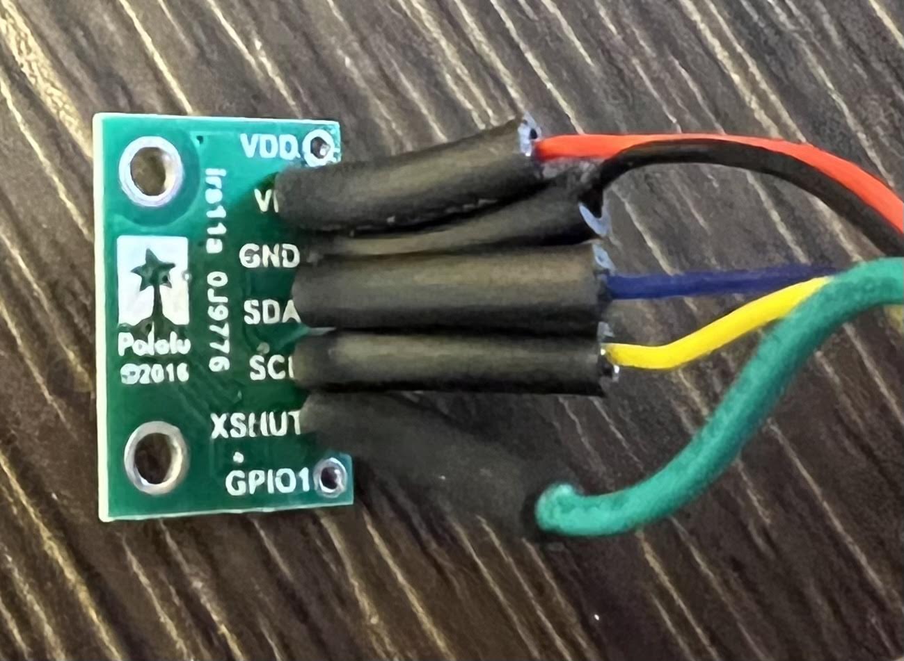
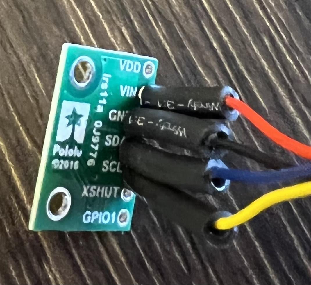
The SparkFun VL53L1X 4m Laser Distance Sensor Library was installed on Arduino IDE. The code to find the I2C address: File->Examples->Apollo3->Wire->Example05_Wire_I2C.ino
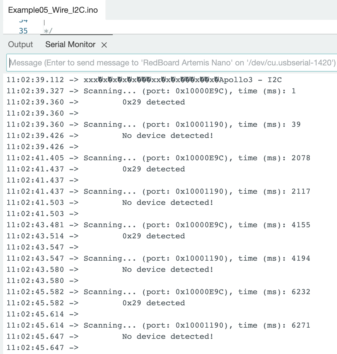
One ToF sensor was connected during the scan. The sensor had an I2C address of 0x29. In the datasheet for the ToF sensor, the listed I2C address is 0x52. The Example05_Wire_I2C.ino code returned an address of 0x29. This is a result of the binary for address 0x52 (binary: 0b01010010) being shifted to the right, resulting in an address of 0x29 (binary: 0b00101001). The rightmost bit is ignored because the bit identifies if data is read/write.
The ToF sensor has two modes: (.setDistanceModeMedium(); //3m has been removed)
Information from the datasheet shows that the short mode can only reach up to 1.3m and is the most resistant to ambient light. The long mode can reach up to 4m but is very sensitive to ambient light, which decreases the distance to 0.73m. The timing budget range for the short mode is 20ms - 1000ms. The timing range for the long mode is 33ms - 1000ms. Short mode has greater accuracy and less sensor noise compared to the long mode. While it would be beneficial for a robot that needs to sense objects farther away to use the long mode, for this lab I am prioritizing accuracy and choose to test the short mode.
The ToF sensor was first tested using the File->Examples->SparkFun_VL53L1X_4m_Laser_Distance_Sensor->Example1_ReadDistance.ino This code was modified to include the line distanceSensor.setDistanceModeShort(); in the setup to choose the short mode for the ToF sensor.
ToF Sensor Setup:
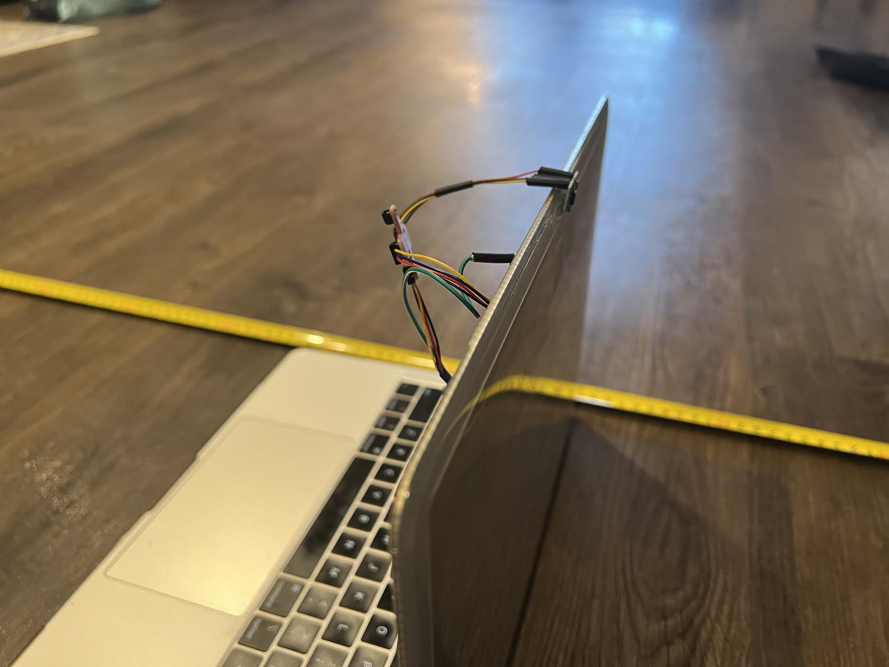
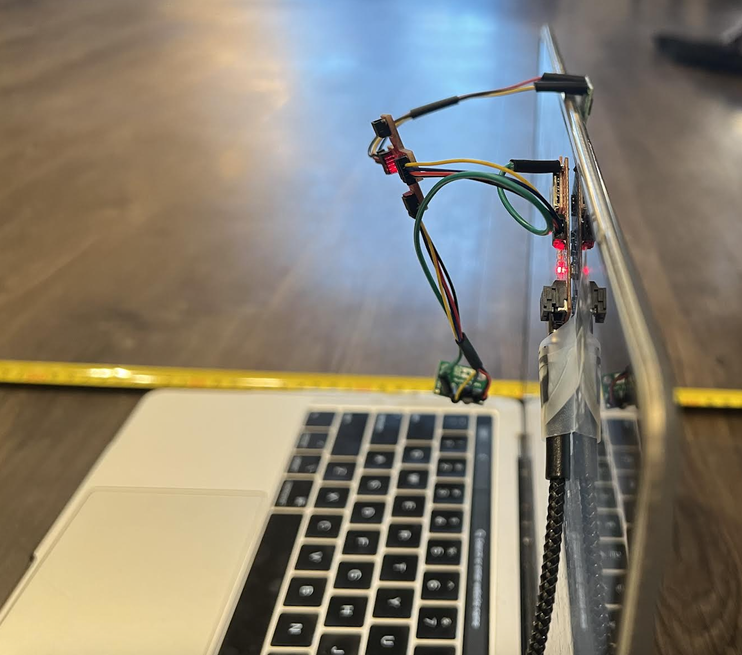
Arudino code to find the ToF distance:
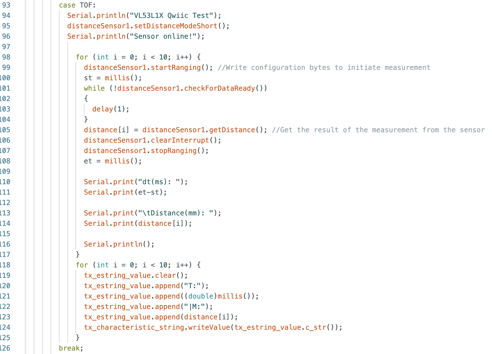
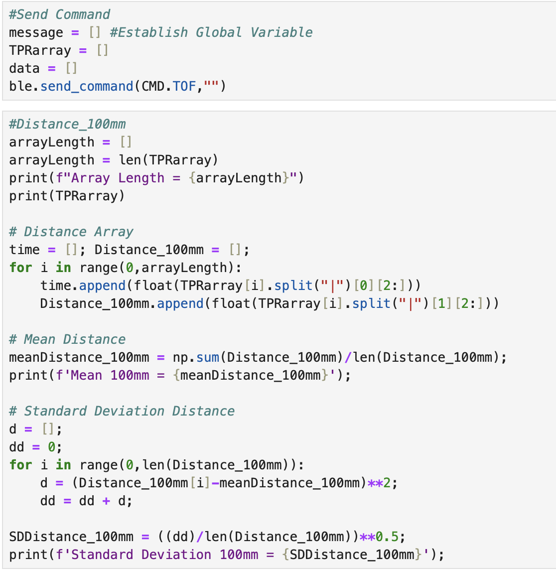
Sensor Range:
In the datasheet it is stated that the short mode for the ToF sensor has a range up to 1.3m. To test the range of the sensor I took an initial measurement at 100mm and continued to take measurements up to 1900mm. The graph below shows the actual distance of the ToF sensor from the wall vs the ToF sensor distance. The plotted measured distance value is the mean value of the ten collected data points. From the graph below it can be seen that after 1.3m the measured values start to differ more from the actual values compared to measured values less than 1.3m.
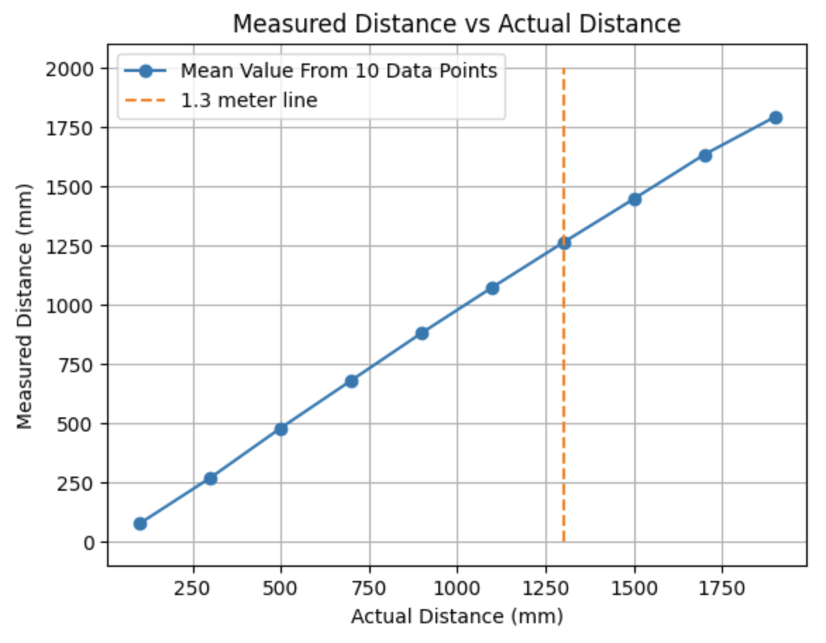
Accuracy:
The difference in the measured and actual distances was plotted against the actual distances the ToF sensor was from the wall. When the ToF sensor is less than 1.3m from the wall, the difference is between 18mm and 40mm. After 1.3m the difference in the measured vs actual distance increases.
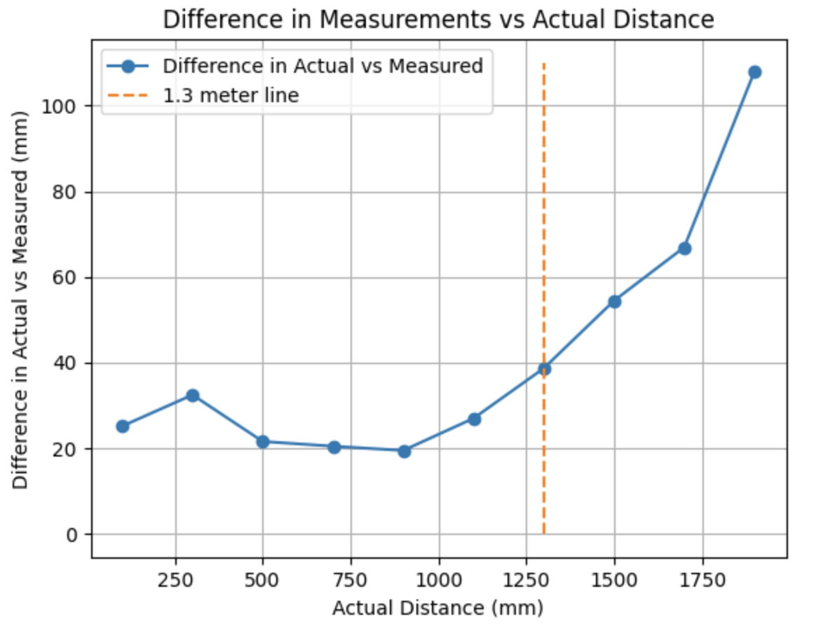
Repeatability:
The standard deviation vs actual distance graph is shown below. The standard deviation is below 3mm for measurements under 1.3m. After 1.3m the standard deviation starts to vary and the standard deviation at 1900mm is 8.75mm.
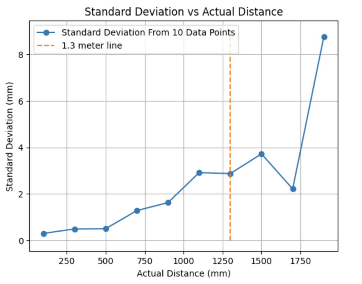
Below are the time and measured distance arrays:
100mm: 9 measurements at 75mm, 1 measurement at 74mm

300mm: 6 measurements at 268mm, 4 measurements at 267mm

500mm: 5 measurements at 478mm, 5 measurements at 479mm

700mm: 5 measurements at 679mm, 4 measurements at 681mm, 1 measurement at 677mm

900mm: 4 measurements at 882mm, 5 measurements at 879mm, 1 measurement at 883mm

1100mm: 5 measurements at 1076mm, 4 measurements at 1070mm, 1 measurement at 1071mm

1300mm: 4 measurements at 1258mm, 4 measurements at 1263mm, 2 measurements at 1265mm

1500mm: 3 measurements at 1448mm, 2 measurements at 1447mm, 3 measurements at 1440mm, 2 measurements at 1449mm

1700mm: 2 measurements at 1634mm, 3 measurements at 1631mm, 3 measurements at 1632mm, 2 measurements at 1637mm

1900mm: 3 measurements at 1782mm, 2 measurements at 1791mm, 4 measurements at 1802mm, 1 measurement at 1784mm

Ranging Time:
The ranging time is the time between each sensor measurement. I commented out all print statements, except the calculated value between the start and end times to allow for code to run as fast as possible. The ranging time was found to be around 55ms.
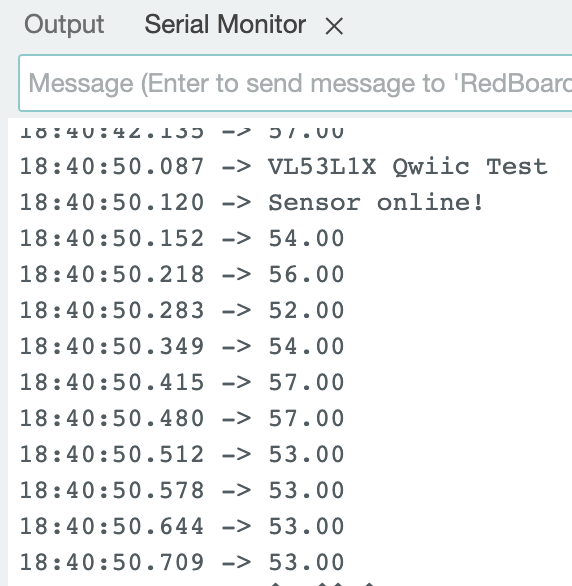
Two ToF Sensors were connected to the Artemis board and Arduino code needed to be written for the two ToF sensors to work in parallel. The code below is written according to the prelab procedure.
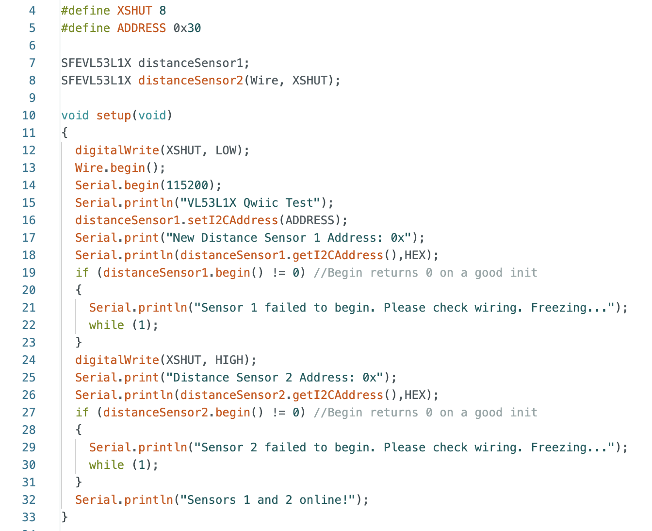
The Serial Monitor prints the I2C addresses for both distance sensors to confirm that one of the addresses was changed to 0x30 and the other remains 0x52.
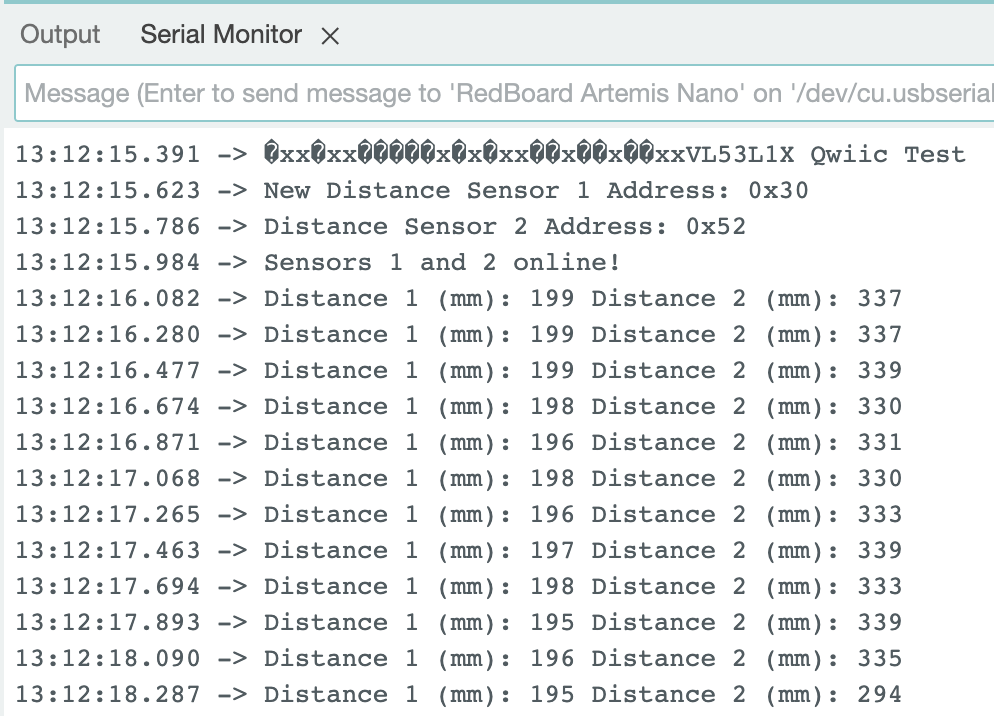
The code to find the ToF sensor speed can be found below. Time is continuously printed and distance measurements are only printed when a measurement is available.
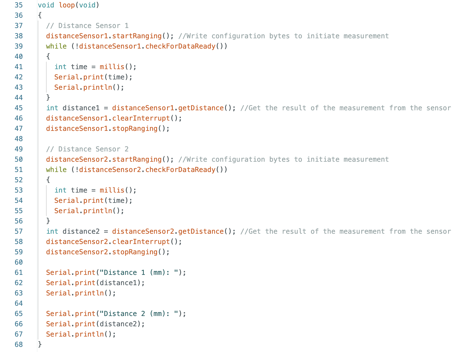
When the sensors are not collecting data the loop takes around 2ms. When data is being collected the loop takes around 11ms. The longer loop time when collecting ToF sensor data is the limiting factor. The limiting factor is the time needed to record distance measurements.
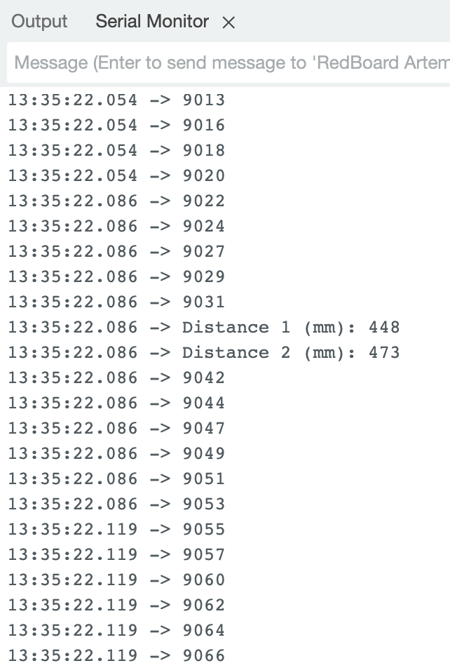
The code from Lab 2 was modified to send time stamped ToF sensor data to Jupyter Notebook. The data for the two ToF sensors was plotted against the recorded time. The case I created in Arduino can be found below.
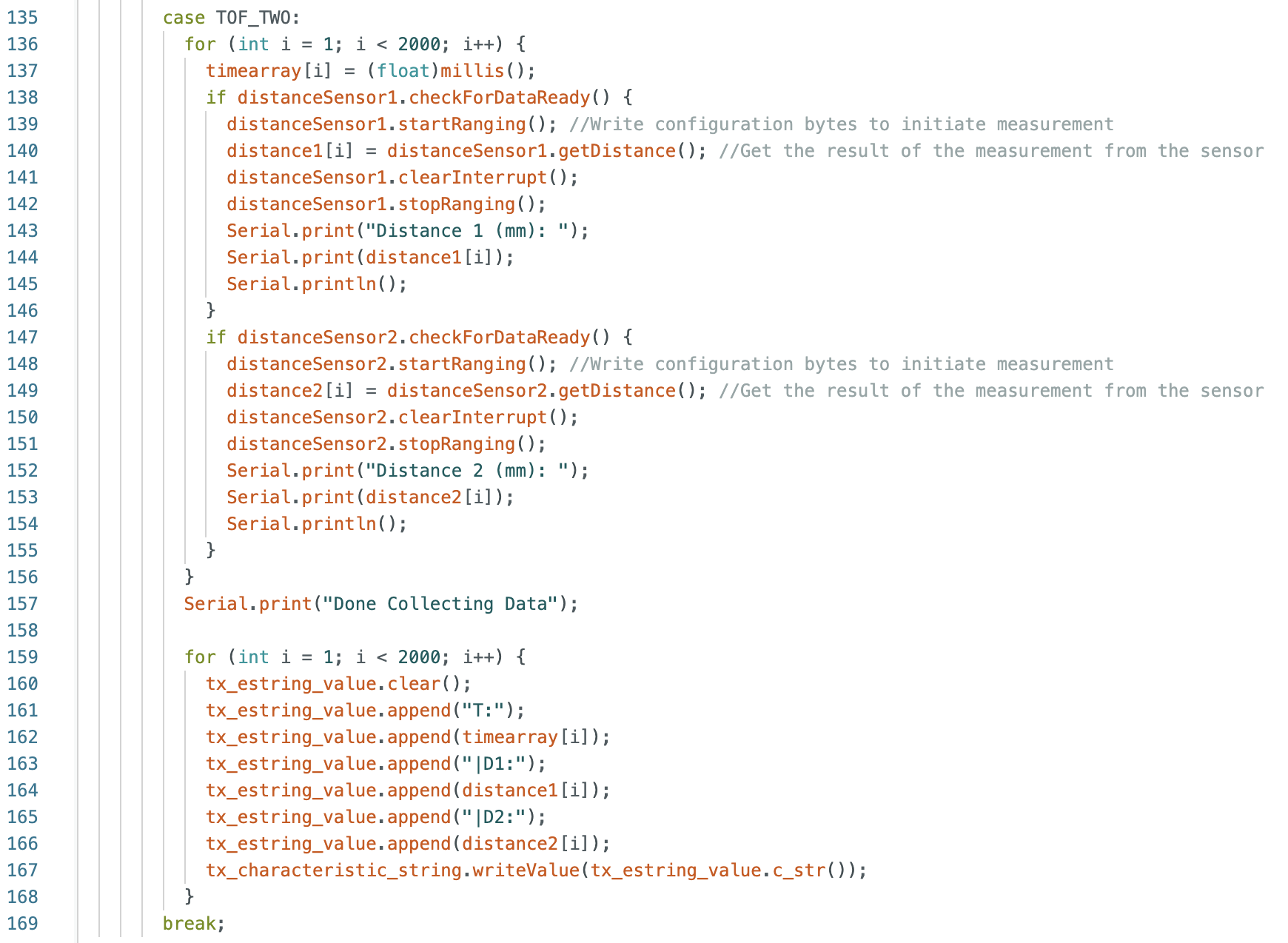
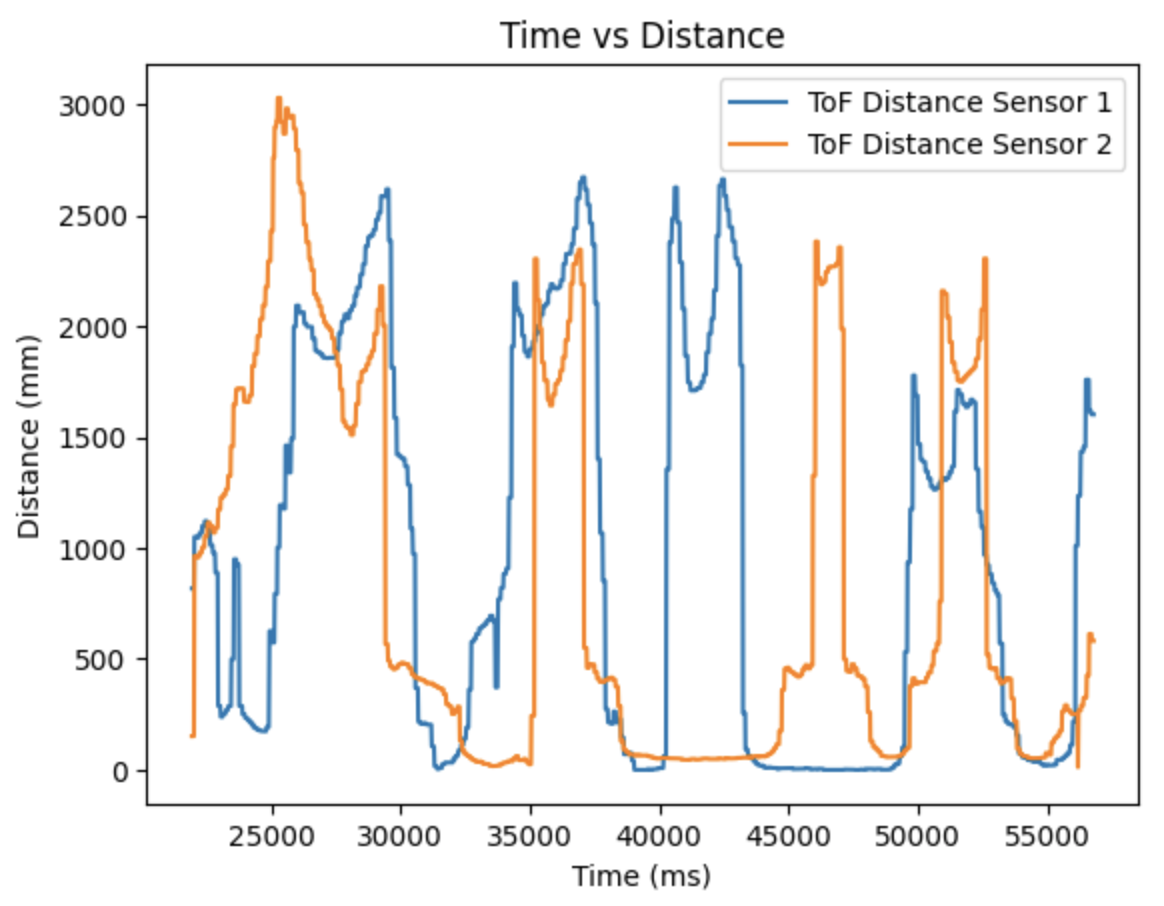
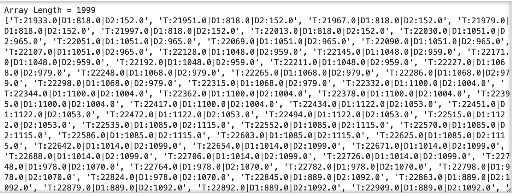
The two main types of infrared sensors are active and passive infrared sensors. Passive infrared sensors sense nearby emitted infrared light, using a difference in signals between two pyroelectric sensors. These sensors are often used for security purposes to detect if there is a heat energy change in the environment, but cannot determine the distance to an object. Active infrared sensors use an emitter and receiver to determine the distance to an object. If there is an obstruction, the active infrared sensor knows that there is an object in between the emitter and receiver. Active infrared sensors are used in industry conveyor belts, as well as in garage door safety mechanisms. (Source: Arrow Electronics) Different types of infrared sensors include proximity sensors, ToF sensors, and triangulation sensors. (Source: NYU)
Four colors and three textures were tested at a distance of 500mm. Colors include pink, blue, yellow, and red. Textures include a hand towel, rug, and folder. The control surface was the dark grey wall that I used throughout the lab for distance readings. The change in color or texture did not affect the ToF sensor's distance output that remained around 478mm.
Control:
Color Pink:
Color Blue:
Color Yellow:
Color Red:
Texture Hand Towel:
Texture Rug:
Texture Folder:
Thank you to all of the TAs that answered my questions. I referenced the past lab reports of Liam Kain, Rafael Gottlieb, Larry Lu, Julian Prieto, and Ignacio Romo.
The objective of the lab is to connect the IMU to the Artemis board and record the robot performing a stunt.
The prelab involved reading about the IMU used in the lab. The lab materials include:
The SparkFun 9DOF IMU Breakout - ICM 20948 - Arduino Library was installed.
The setup for this lab is shown in the image below.
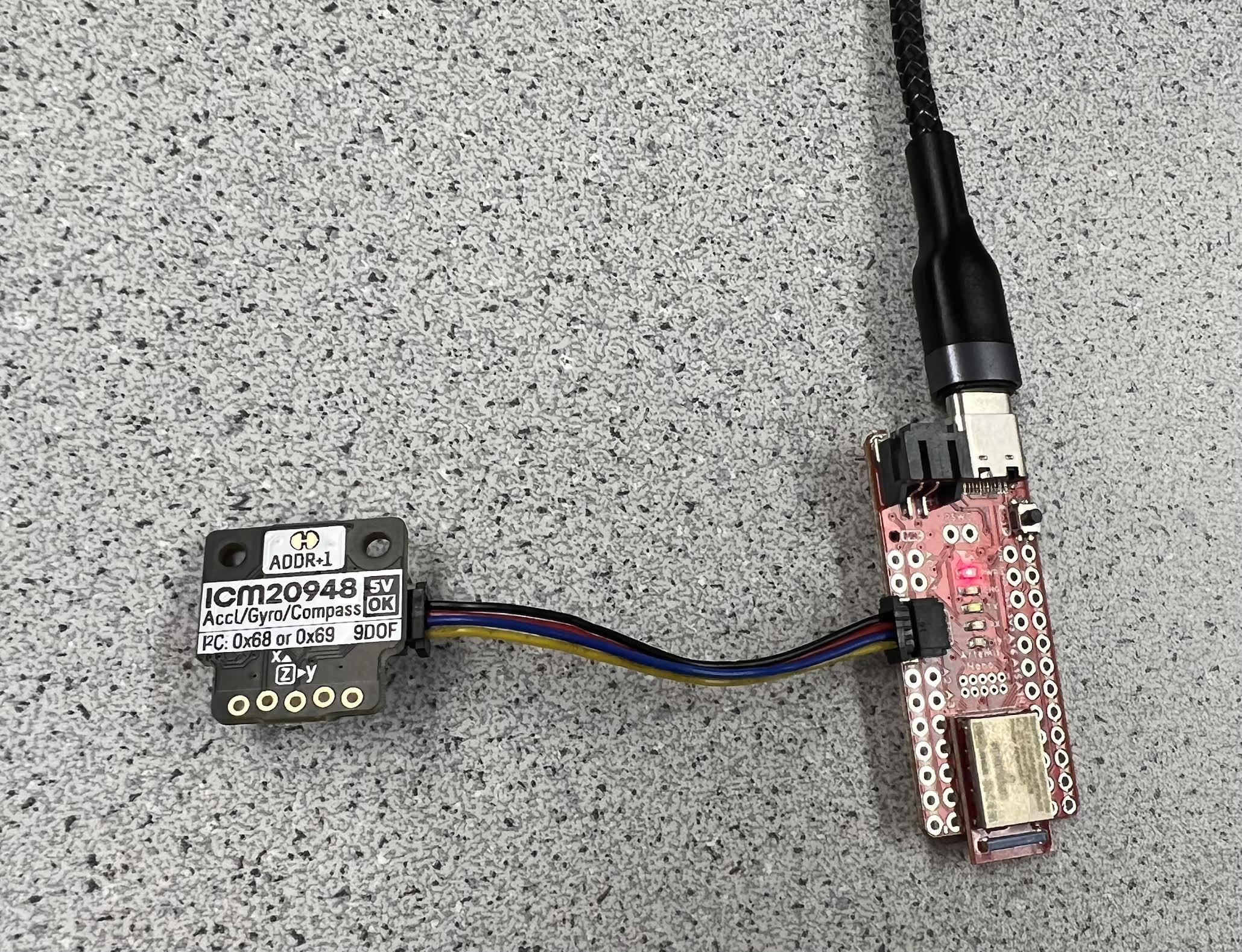
The example code found under SparkFun 9DOF IMU Breakout - ICM 20948 - Arduino Library->Arduino->Example1_Basics was run to test if the IMU was working correctly.
Upon opening the Example1_Basics code, the AD0_VAL default was set to one. When the ADR jumper is closed the value should be set to zero. AD0_VAL corresponds to the last bit of the I2C address. My ADR jumer on the IMU was closed. For this reason, I needed to change the AD0_VAL to zero to return the accelerometer, gyroscope, magnetometer, and temperature data.
While viewing the output data in the serial monitor, I moved the IMU to change the accelerometer and gyroscope data. I looked at the notated axis that was printed on the IMU and moved the IMU along the X, Y, and Z axis. I noticed that the respective X, Y, and Z serial monitor outputs for the accelerometer increased when I moved the IMU along the respective positive axis. The gyroscope data for pitch, roll, and yaw also changed when I rotated the IMU around the X, Y, and Z axis.
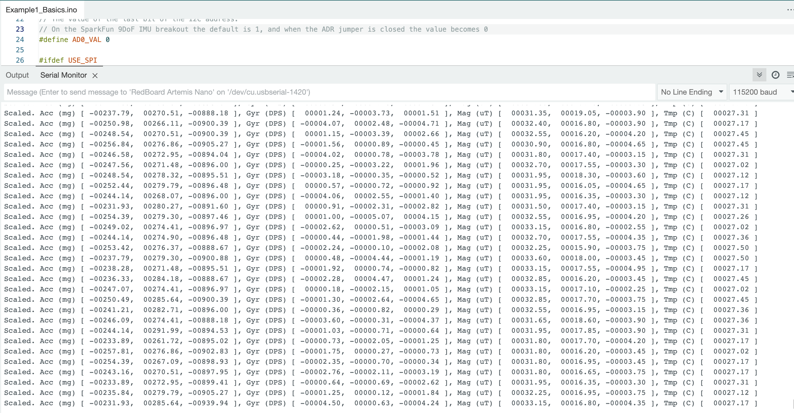
In the Example1_Basics code, I added a slow blink at the beginning of void setup() to turn the Artemis LED on and off three times.
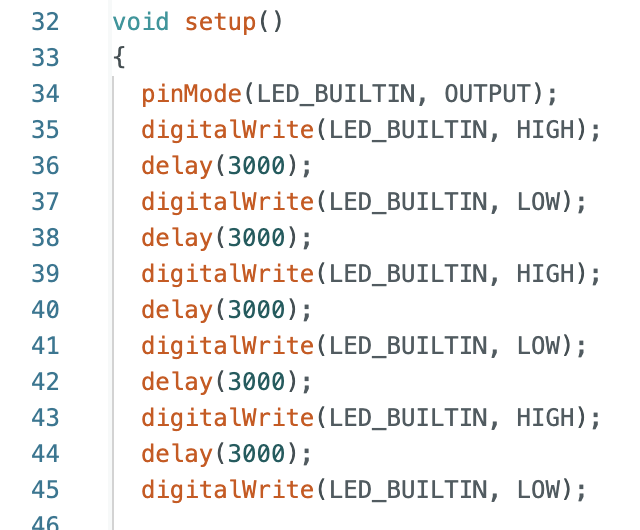
The following equations for pitch (theta) and roll (phi) were found in the FastRobots-4-IMU Lecture Presentation.
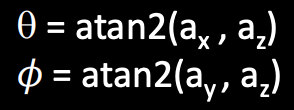
These equations were used to compute pitch and roll for the accelerometer. I implemented the calculations in the Example1_Basics sketch (lines 247 - 255 below) that was used in the previous task to receive continuous data from the Artemis board and plot the results.
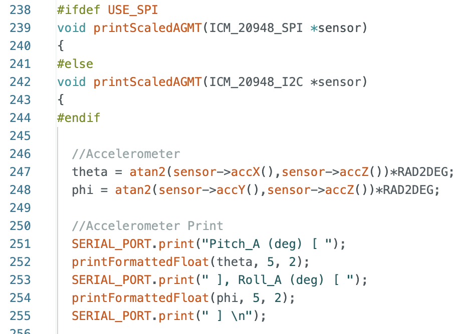
The below graphs show Pitch (data 0, green) and Roll (data 1, purple) at 0 degrees. The x-axis is time (sec) and the y-axis is degrees.
Pitch and Roll at 0 degrees:
.png)
The below graphs show Pitch (data 0, green) at -90 and 90 degrees and the corresponding Roll (data 1, purple) outputs. The x-axis is time (sec) and the y-axis is degrees. From the graphs it can be seen that when pitch is at -90 degrees there is noise in the roll outputs.
Pitch at -90 degrees:
.png)
Pitch at 90 degrees:
.png)
The below graphs show Roll (data 1, purple) at -90 and 90 degrees and the corresponding Pitch (data 0, green) outputs. The x-axis is time (sec) and the y-axis is degrees.
Roll at -90 degrees:
.png)
Roll at 90 degrees:
.png)
I plotted the data for pitch and roll at 0, 90, and -90 degrees in Jupyter Notebook and calculated the mean and standard deviation.
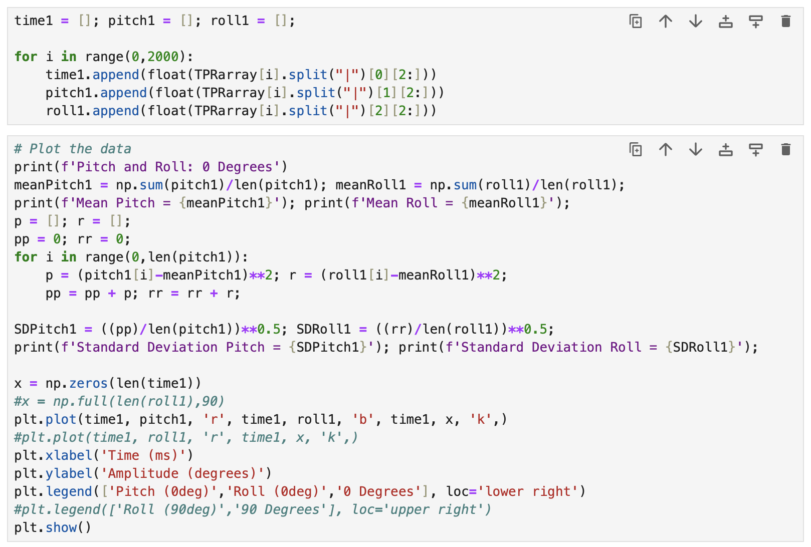
Below are graphs. I also included a black line at 0, 90, or -90 degrees for reference. Note: The data for the graphs was collected by holding the IMU against the table using my hand. This may have resulted in some error due to the surface level or any small hand movements. In the future the IMU should be calibrated when it is secured to the robot to achieve the most accurate pitch and roll data.
Analysis.png)
.png)
.png)
.png)
.png)
The noise in the accelerometer was examined using a Fast Fourier Transform. Data for the FFT was collected as I moved the IMU. The sinusoid and the FFT graphs can be found below. There is a large spike closer to 0Hz and less noise as the frequency increases. Note: I modified the code from Stephan Wagner's Ed Discussion post to plot the FFT graphs.
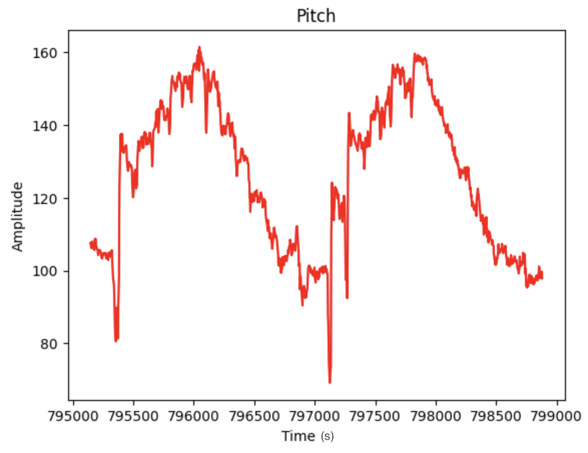
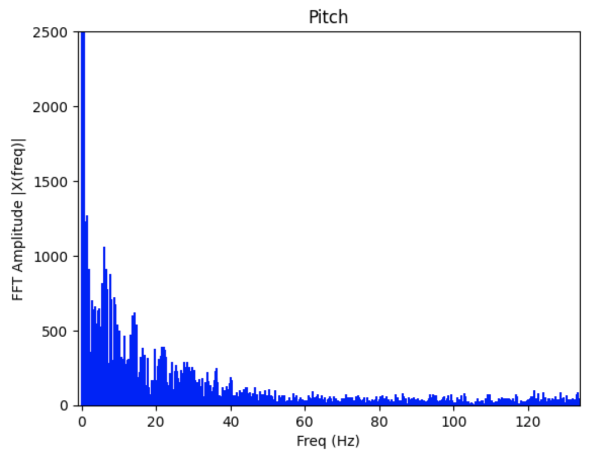
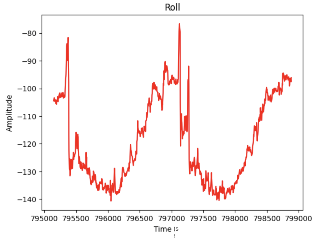
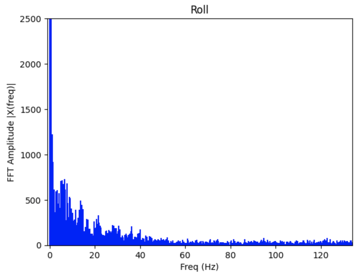
From observing the above graphs, I choose a cutoff frequency of 25Hz to use for a low pass filter. Using the determined cutoff frequency, I calculated the alpha used in the low pass filter. The equations from lecture are below:
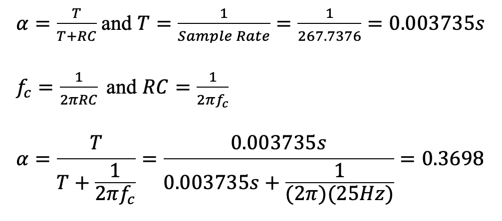
The low pass filter alpha was calculated to be 0.3698
The low pass filter was implemented in Arduino. The code to find pitch and roll for the accelerometer can be found below.
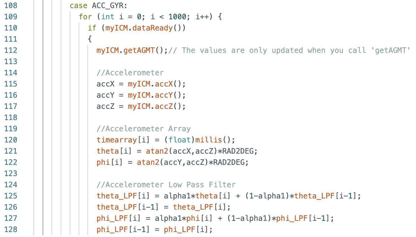
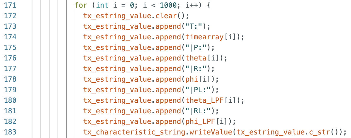
The below FFT graphs show the original signal (red) and the reduction in noise after implementing a low pass filter (blue). Choosing a lower cut off frequency reduces more noise.
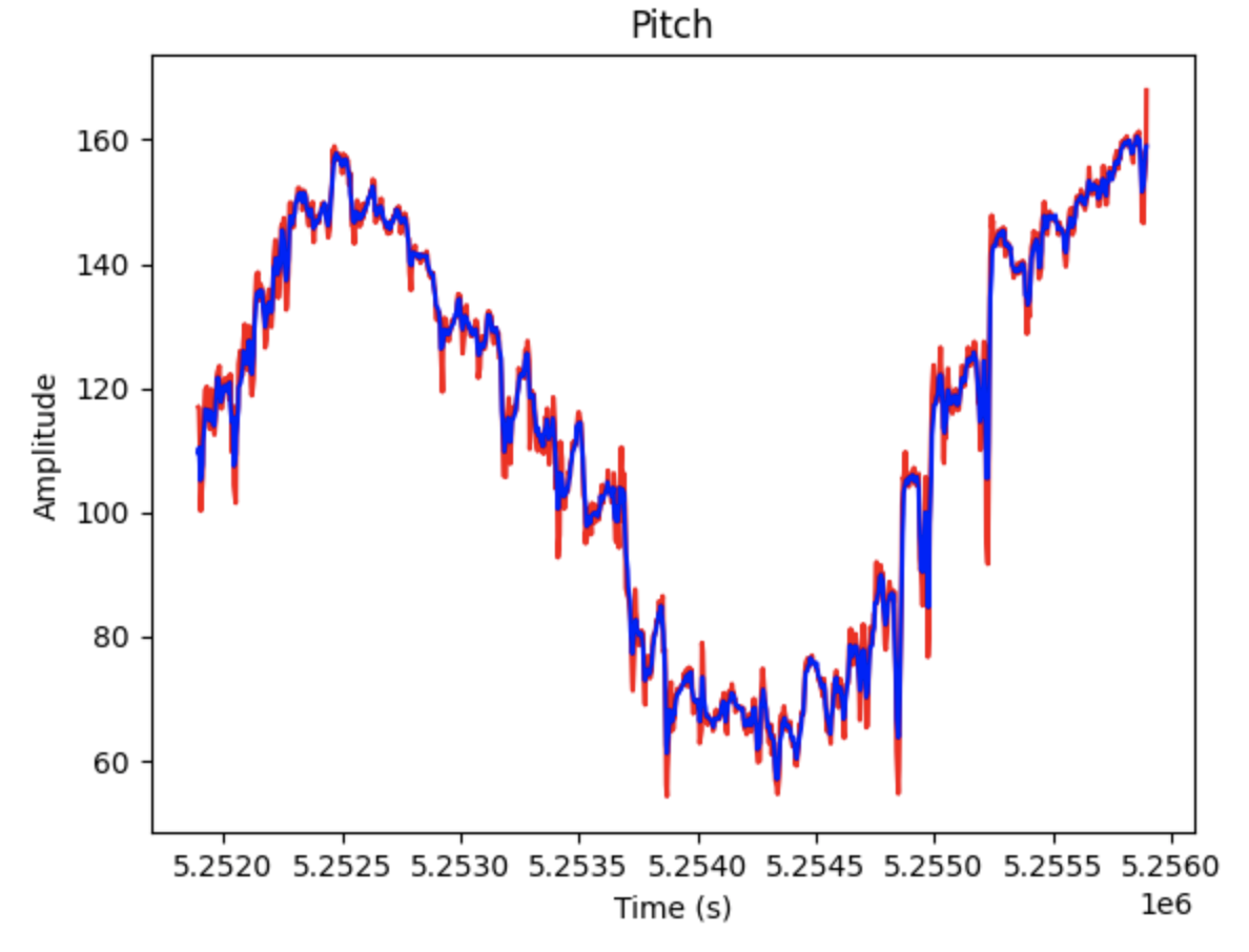
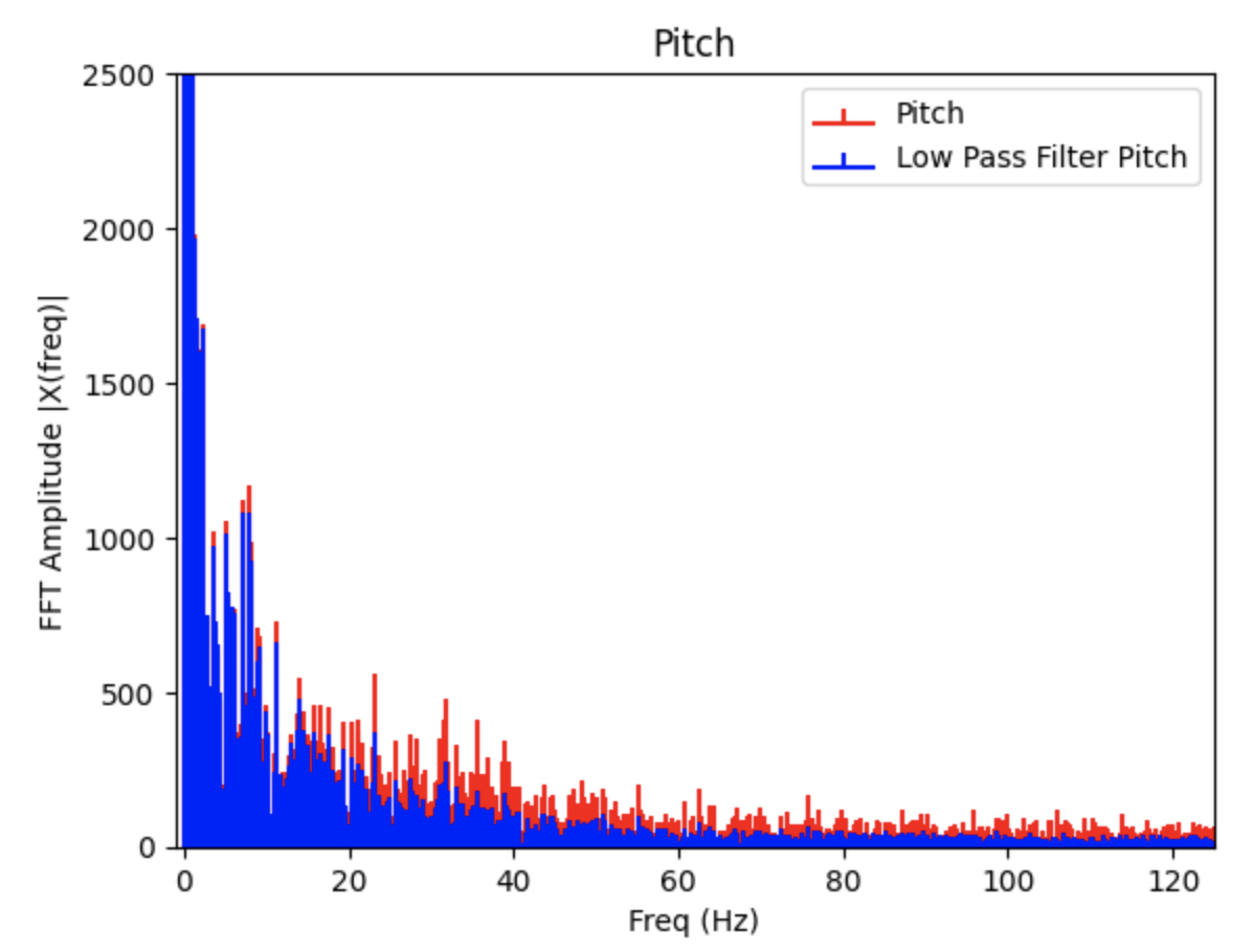
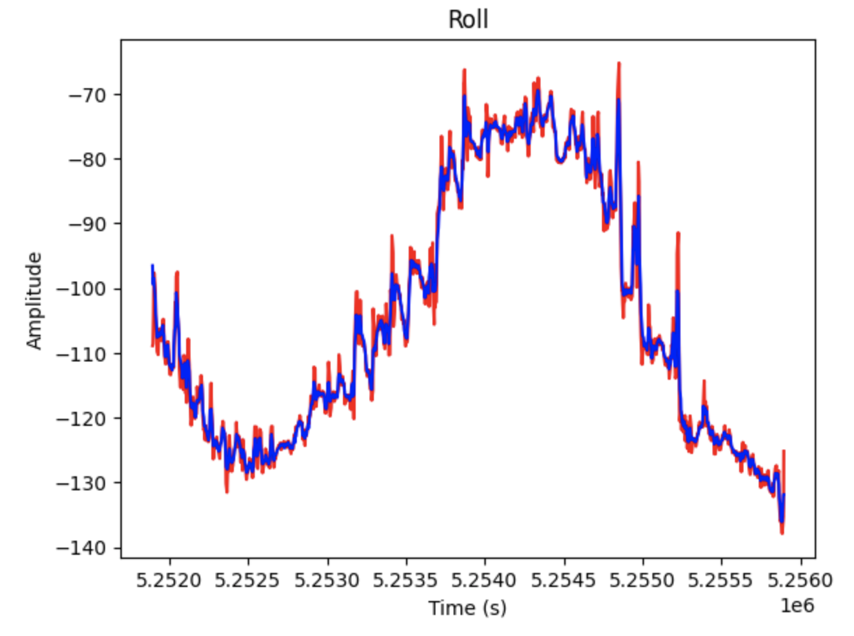
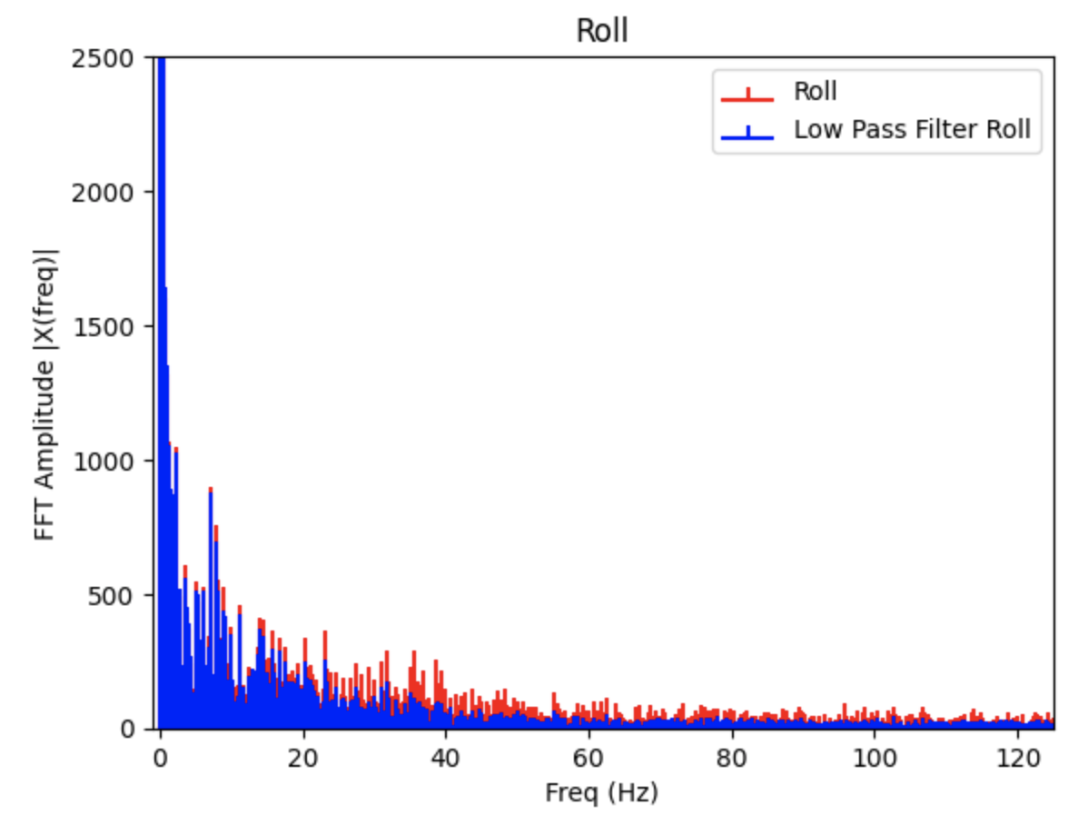
Prior to implementing a low pass filter, there was not a significant level of noise in the IMU data due to a pre-existing internal low pass filter. The information for this can be found on page 10 of the datasheet for the IMU.

The following equations for pitch, roll, and yaw were found in the FastRobots-4-IMU Lecture Presentation.

The gyroscope measures angular velocity. To find pitch, roll, and yaw the data collected from the IMU needs to be multiplied by a time step (dt in the below code).

The code above was added to Example1_Basics and plotted alongside the data for the accelerometer's pitch and roll. The gyroscope data drifts over time, but has less noise then the accelerometer data. In the below graphs the IMU was moved slightly to achieve different outputs.
Pitch for Gyroscope (Blue) and Accelerometer (Orange):
Roll for Gyroscope (Blue) and Accelerometer (Teal):
The drift for the gyroscope can be better seen in the below graphs. The gyroscope was held in the same position as the data was collected. As time increases the measurements drift away from the starting value.
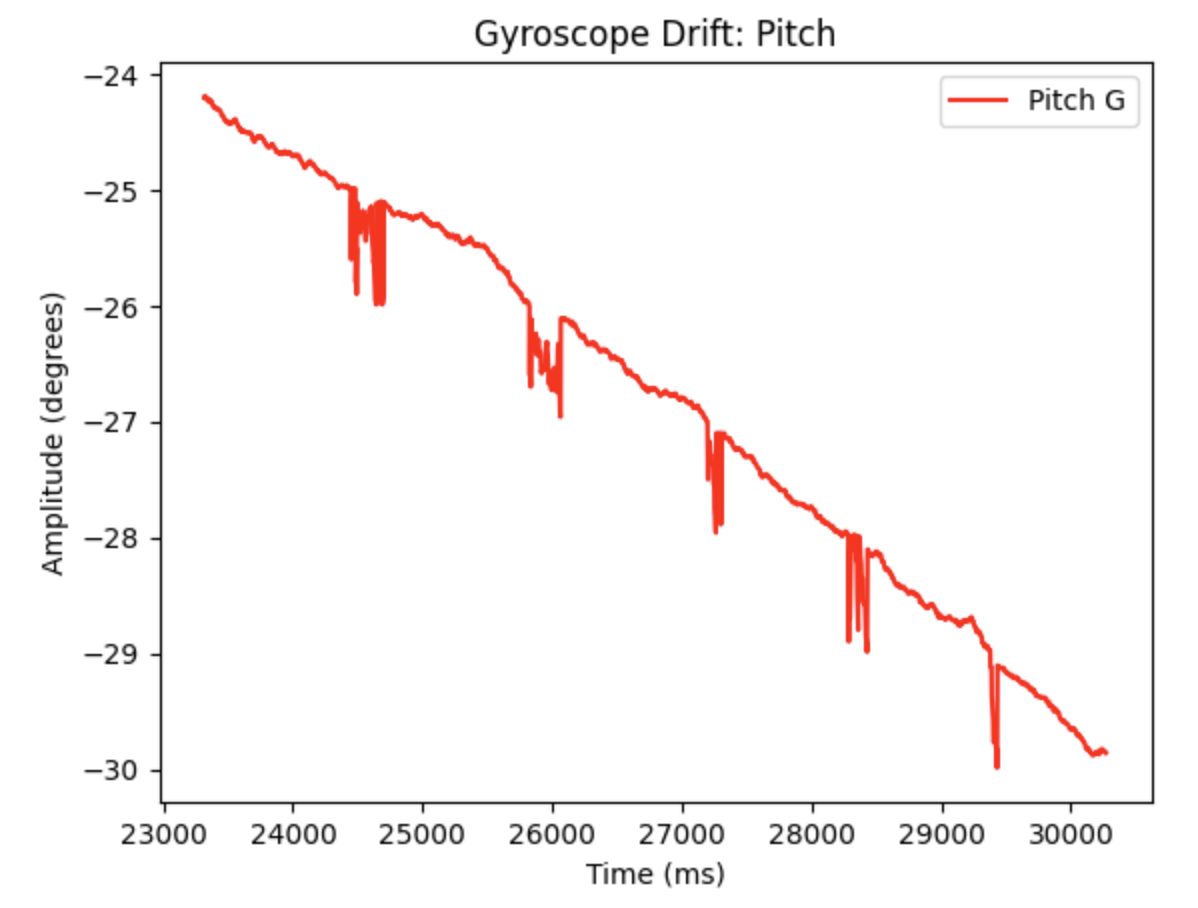
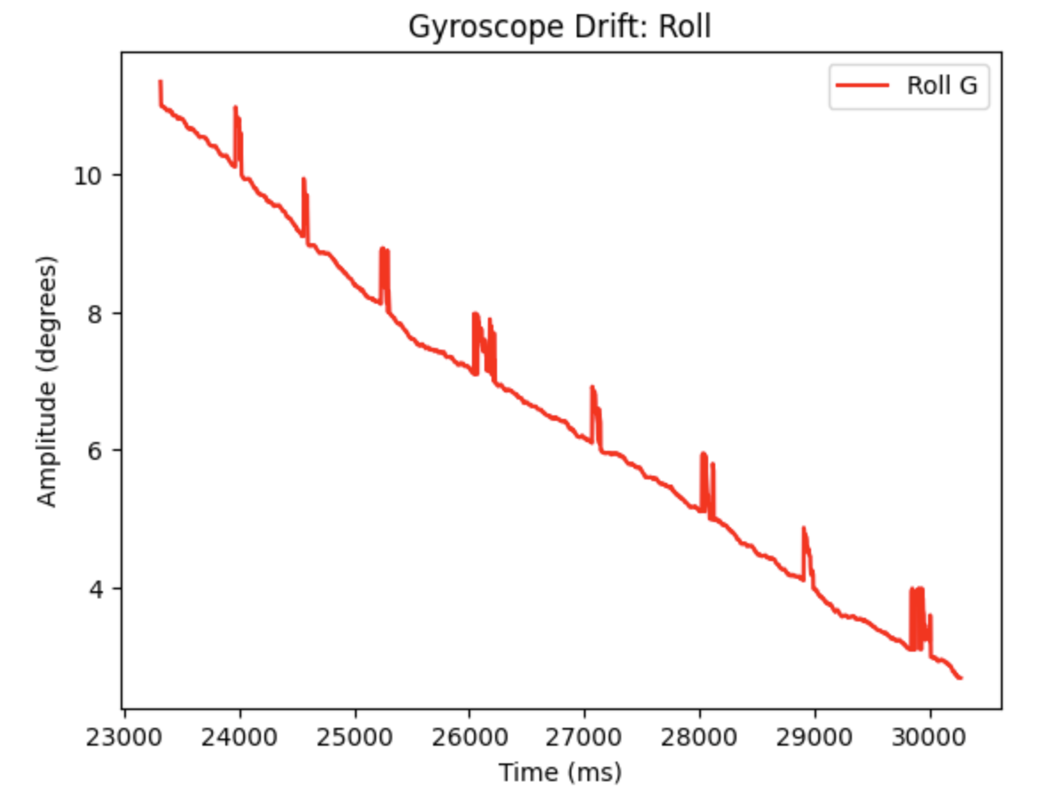
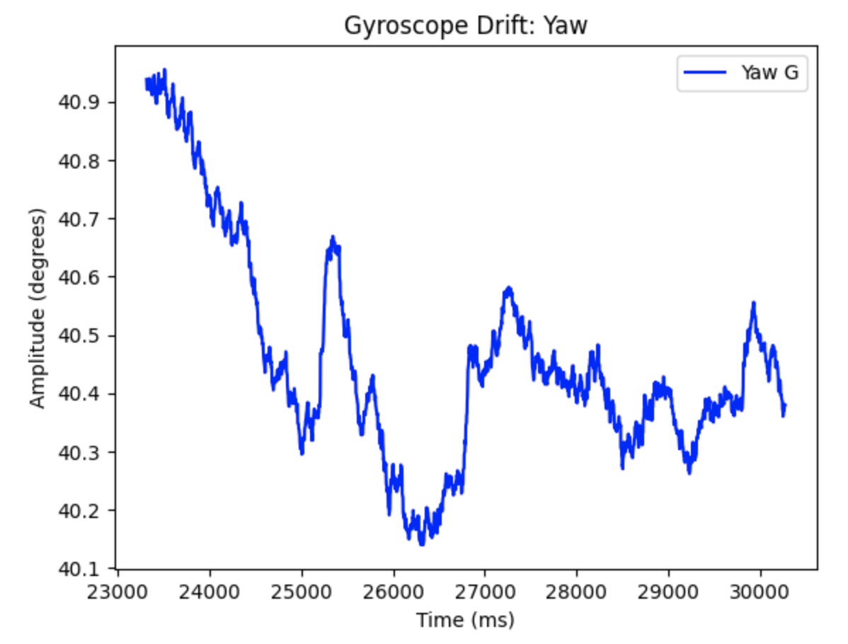
Code to plot the above graphs:
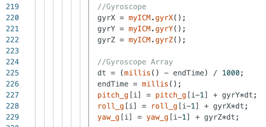
Decreasing the sampling frequency resulted in a slower update to the angle measurements and more variation in the outputs between each successive measurement. The sample rate should be high to achieve the greatest level of accuracy when recording data.
Complimentary filter equation from lecture:


The complimentary filter shows resistance to small vibrations as the IMU is moved during data collection. The complimentary filter reduces noise compared to the accelerometer output. Alpha is a set constant that represents how well the accelerometer output measures the correct pitch and roll data. I examined how different alpha values affected the graphs. In the below graphs alpha = 0.5
Pitch for Gyroscope (Blue), Gyroscope Complimentary Filter (Orange), and Accelerometer (Teal):
Roll for Gyroscope (Blue), Gyroscope Complimentary Filter (Orange), and Accelerometer (Teal):
Pitch for Gyroscope, Gyroscope Complimentary Filter, and Accelerometer (alpha = 0.5):
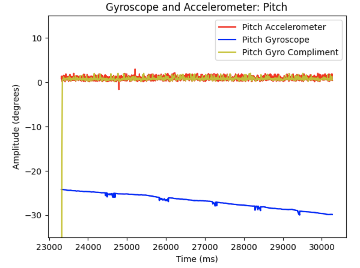
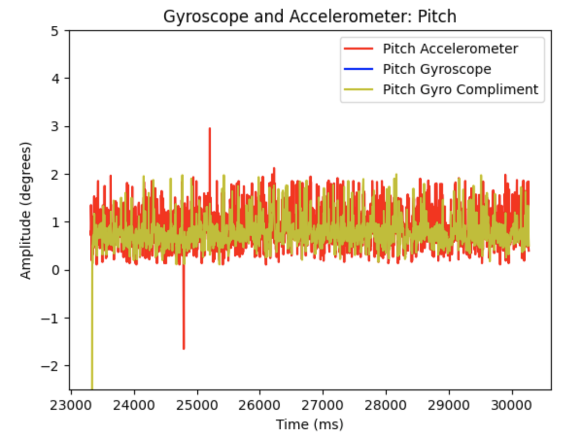
Roll for Gyroscope, Gyroscope Complimentary Filter, and Accelerometer (alpha = 0.5):
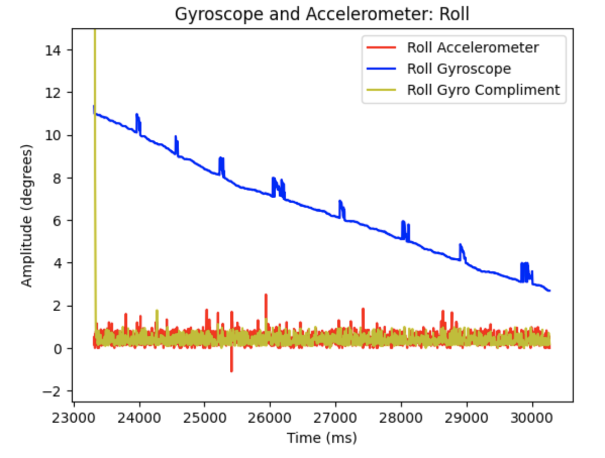
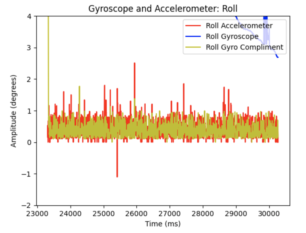
Additional graphs when alpha = 0.2
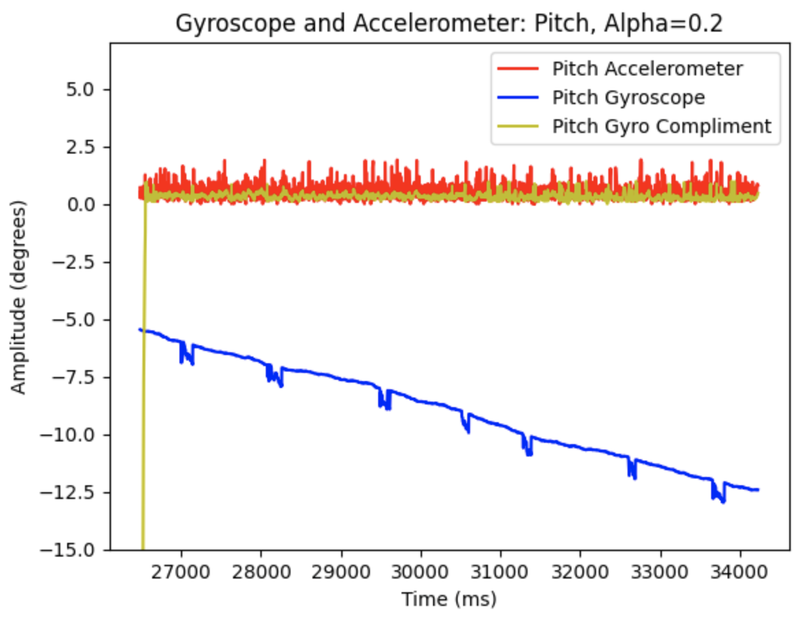
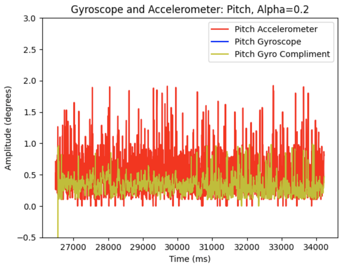
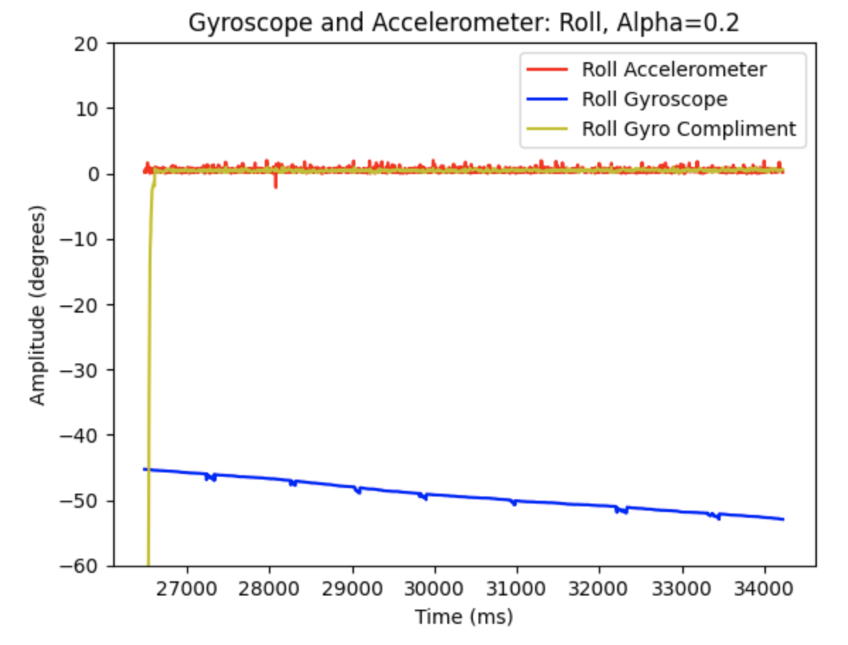
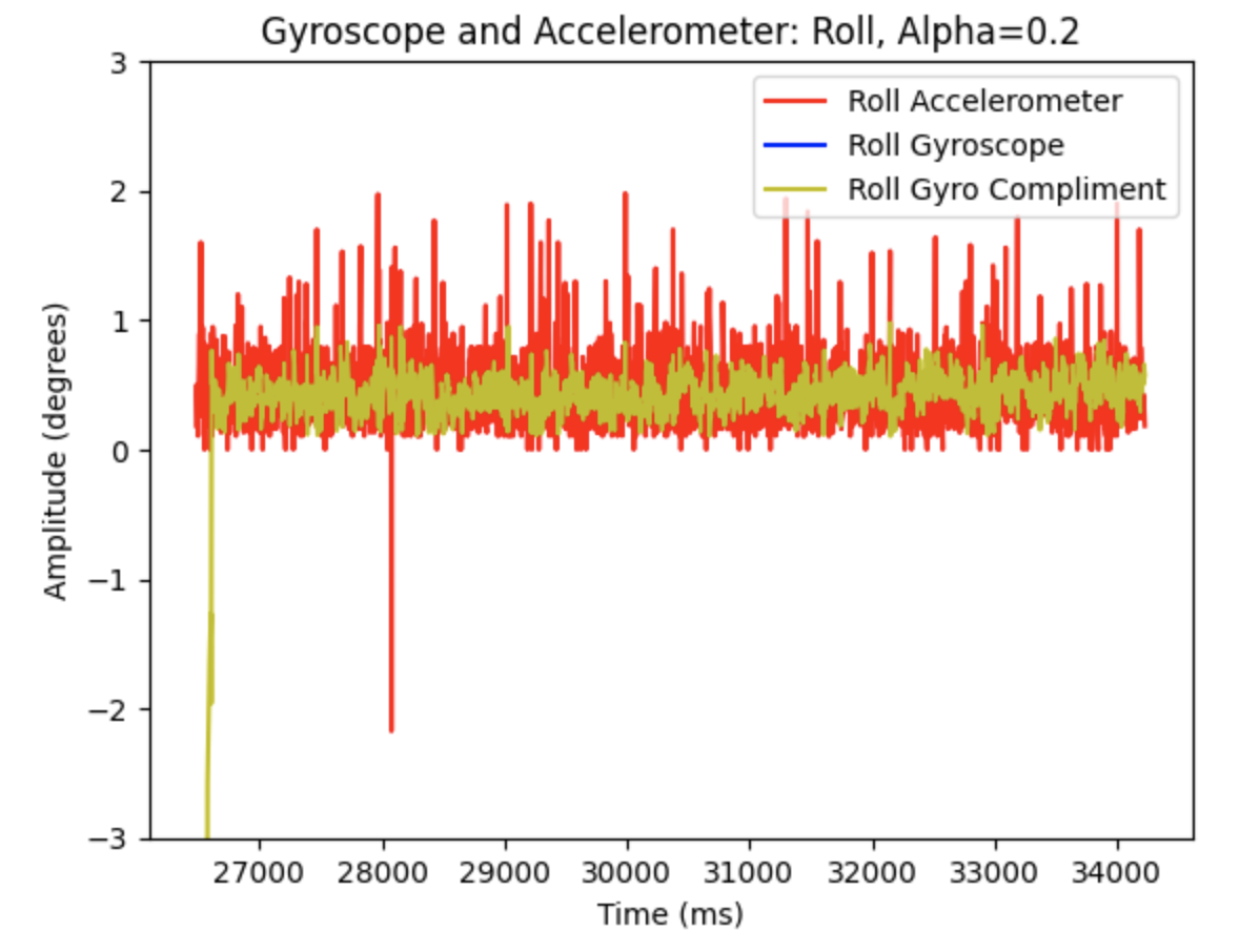
Code to plot the above graphs:

All of the accelerometer and gyroscope data print statements and any delays in the ble_arduino.ino file were removed in order to speed up the execution of the main loop. A case called "ACC_GYR" was created that checked if the data was ready in the main loop, and if there was data available stored it in arrays. After speeding up the loop I found that new values were sampled every 0.04s, which is a sampling frequency of 1/0.04s = 25Hz.
The data is stored in arrays on the Artemis board before being sent to Jupyter Notebook. There are 7 arrays including time (1); accelerometer: x (2), y (3), z (4); gyroscope: x (5), y (6), z (7). I choose to use separate arrays because in the future I can decide what data I want to send to Jupyter Notebook. The data type used to store the data is a float. I choose to use a float as it is less bytes then a double, allowing for more data to be stored on the memory of the Artemis. A float is 4 bytes, resulting in one packet of data information for the 7 arrays to be 28 bytes. The Artemis has 384kB of RAM. Sampling at 0.04s (25Hz) will result in data being collected for 548 seconds.
Code to find X, Y, and Z for Accelerometer and Gyroscope.
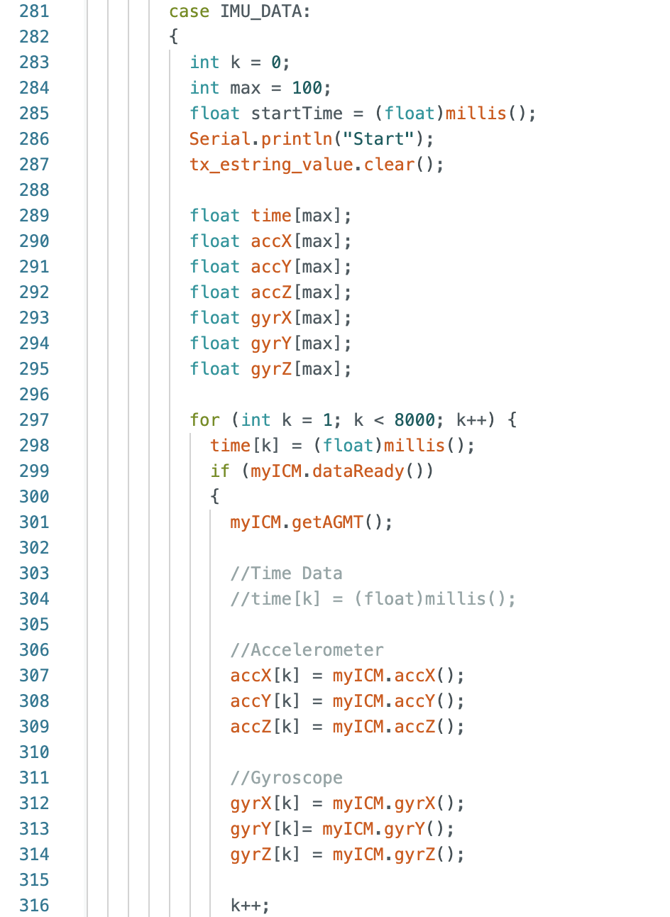
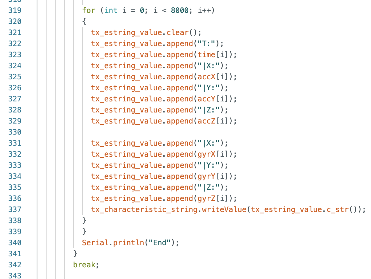
Code to find pitch and roll for Accelerometer; and pitch, pitch compliment, roll, roll compliment, and yaw for Gyroscope.
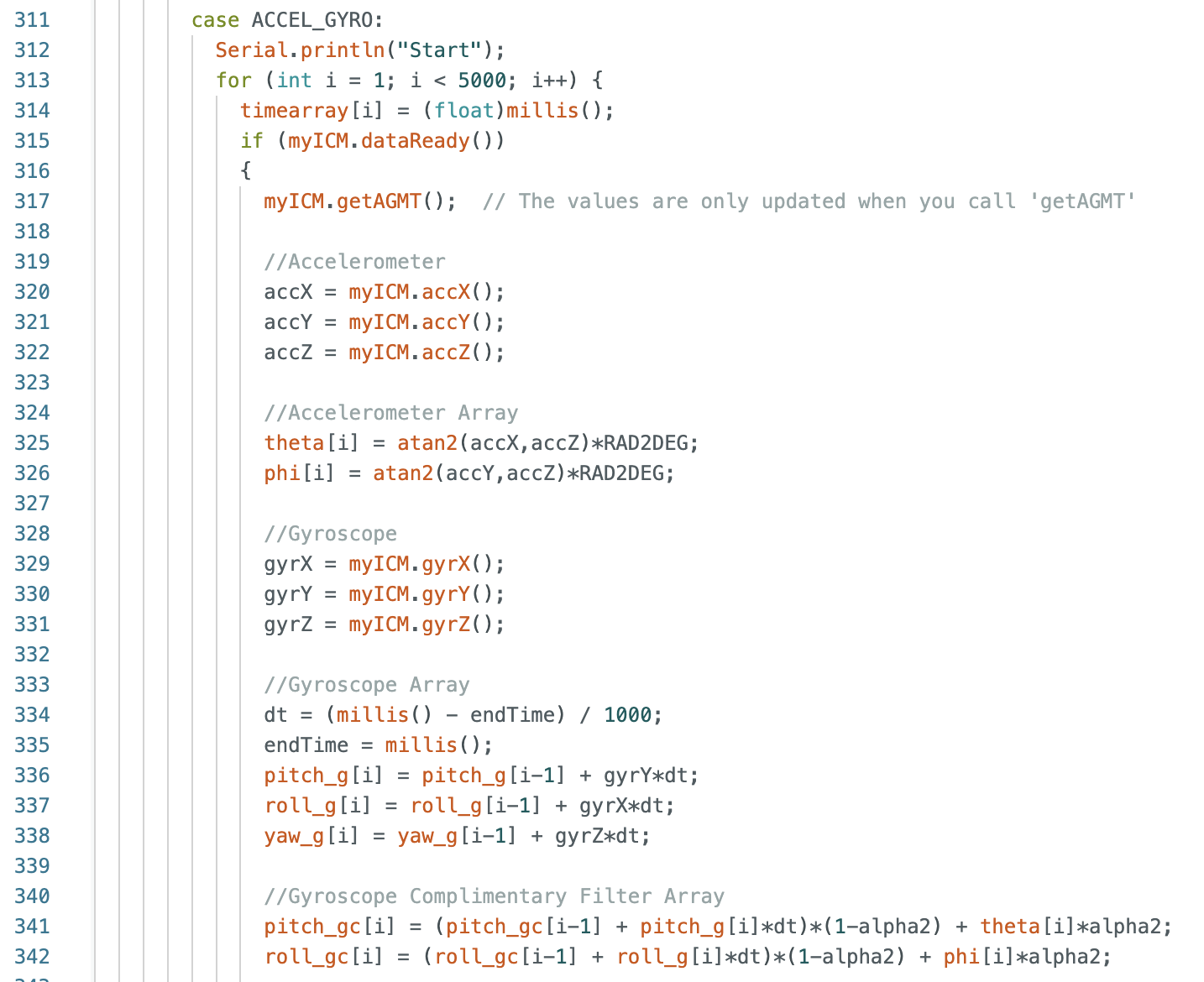
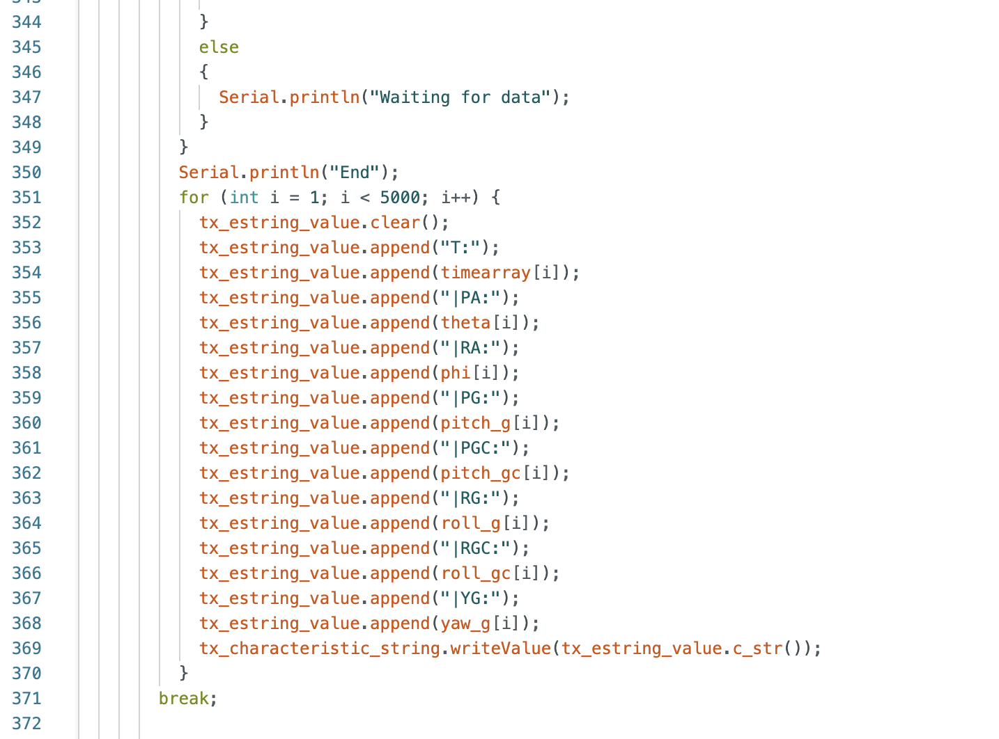
I collected data for the X,Y,Z positions of the accelerometer and gyroscope as well as the pitch and roll for the accelerometer; and pitch, roll, and yaw for the gyroscope.
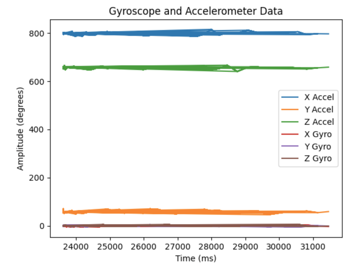
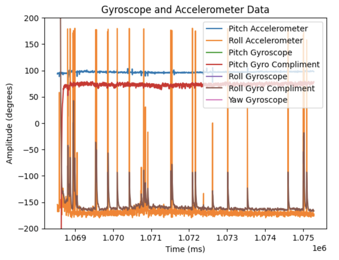
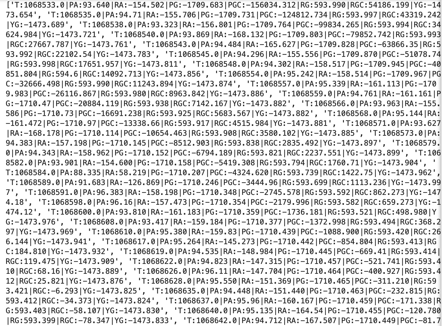
The robot is moved using the controller. The robot can move very quickly, but it is hard to control the speed. If the robot changes directions too quickly there is a chance that it might flip over. It is also hard to slow down the robot to a stop. When slowing down the robot, the reverse needs to be applied. This is easy to over compensate and the robot might end up traveling in reverse rather than coming to a stop.
Thank you to all of the TAs that answered my questions. I referenced the past lab reports of Liam Kain, Rafael Gottlieb, Larry Lu, Julian Prieto, and Ignacio Romo.
Test the connection between the Artemis board and the computer. Arduino IDE was installed and a number of tasks were completed to show the functionality of the Artemis board.
Arduino IDE 2.2.1 was installed onto my computer.
Materials include:
Better Serial Plotter was installed to plot the temperature in Task 4.
The instructions for Arduino Installation were followed to ensure proper connection between the Artemis board and the computer. The SparkFun Apollo3 Boards package was installed using the Boards Manager in Arduino IDE (shown below).
The first task involved a blinking LED on the Artemis board. Example code: File->Examples->01.Basics->Blink. A loop was implemented and used the function digitalWrite() to turn on the LED for one second and then turn off the LED for one second (shown below).
In this example serial communication between the Artemis board and the computer was tested. Example code: File->Examples->Apollo3->Example04_Serial.
Below is an image and video of the Serial Monitor showing the outputs: "Hello", "This is the serial example", "Test 1", "Test 2", and "Test 3".
The temperature sensor of the Artemis board was tested. Example code: File->Examples->Apollo3->Example02_AnalogRead. I covered the sensor with my hand to increase the temperature reading. At the beginning of the test the temperature is around 32.3 degrees Celsius and reaches a temperature of around 33.4 degrees Celsius (shown below).
Another example shows various temperatures being plotted using Better Serial Plotter.
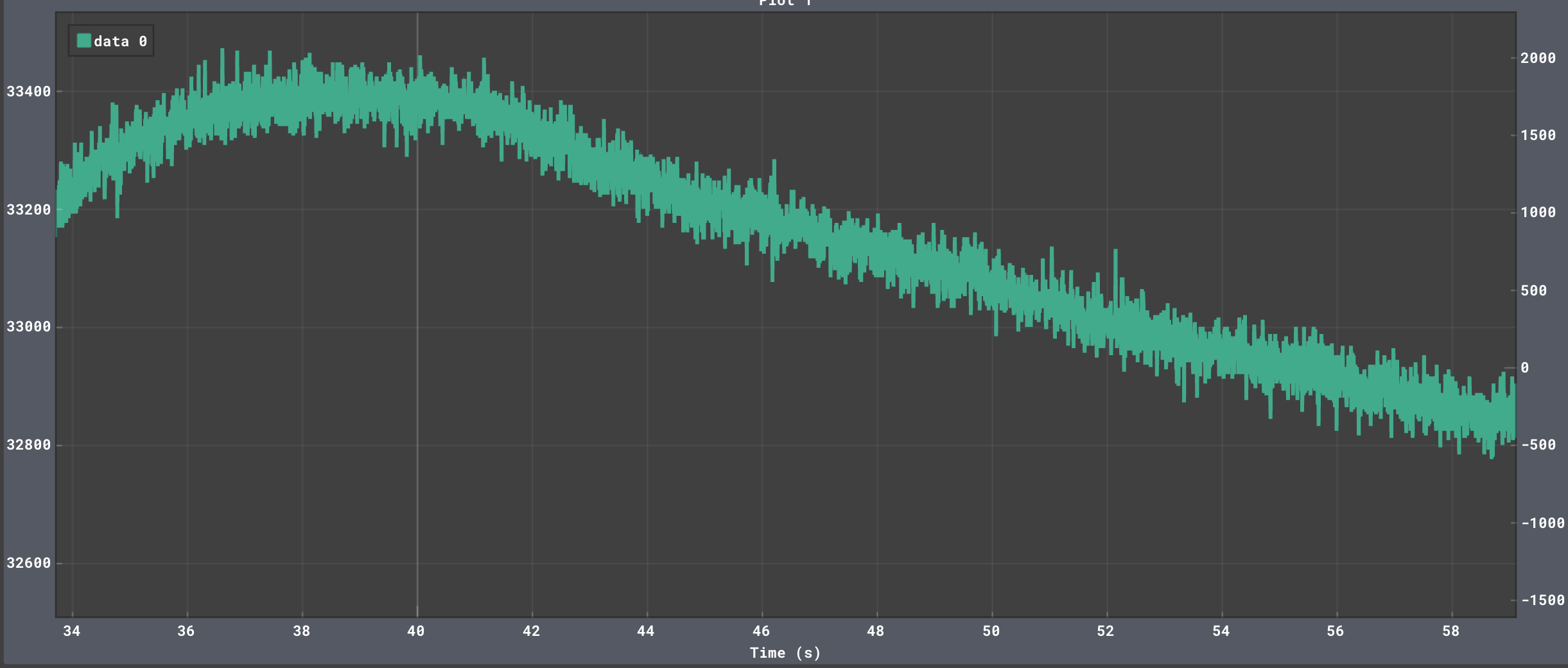
The Microphone Output task tests the microphone of the Artemis board. Example code: File->Examples->PDM->Example1_MicrophoneOutput. During this task I spoke into the microphone to change the frequency (image and video shown below).
The Artemis board was programmed to turn on the LED when the musical note A4 is played on a speaker (code below). I started with the Example01_MicrophoneOutput sketch, and I added if statements (lines 113-122 below). The note A4 is 440Hz (UC Berkeley Reference). The first if statement determines if the frequency is between 430Hz and 450Hz to account for any slight error in sound quality. If the frequency is within range an “A4” statement will be displayed in the Serial Monitor and the LED on the Artemis board will turn on. The second if statement determines if the frequency is lower than 430Hz or greater than 450Hz. If the frequency is lower than 430Hz or greater than 450Hz a “Not A4” statement will be displayed in the Serial Monitor and the LED on the Artemis board will turn off.
Image of the outputs in the serial monitor:
Video showing the LED turning on when the note A4 is played:
I added to the LED and Musical A4 task by creating a musical tuner. There are eleven total if statements that determine the note being played (lines 113-168 below):
Video of various notes being played:
I tested the connection between the Artemis board and the computer. Tasks performed included turning on and off an Artemis board LED, printing serial monitor outputs, viewing temperature data in the serial monitor, testing the microphone, and creating a musical tuner.
Tested the Bluetooth communication between the computer and the Artemis board. Python in a Jupyter Notebook was used for the computer and Arduino IDE was used for the Artemis board.
During the setup for the lab I already had installed Python 3. I needed to install pip by running the line "python3 -m pip install --user virtualenv" in the Command Line Interface (CLI). I created a folder called “MAE 5190 Lab” where I put all of the Jupyter Notebook files. I then created a virtual environment by typing "python3 -m venv FastRobots_ble" in the CLI.
The virtual environment was activated by typing "source FastRobots_ble/bin/activate" and then deactivated by typing "deactivate".
The python packages were installed by entering "pip install numpy pyyaml colorama nest_asyncio bleak jupyterlab" into the CLI.
CLI entered commands:


I also needed to install matplotlib to use for the 5000 level tasks. I asked a TA for help with the installation. Below is a picture of the command entered into the CLI.
To import modules into the Jupyter Notebook the following lines of code were run.
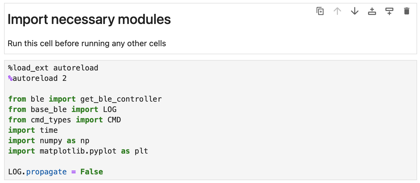
After uploading the provided ble_ardunio.ino file to the Artemis board the MAC address was printed in the serial monitor. The MAC address is c0:83:34:6a:b2:3c The image below shows the Arduino serial monitor with the printed MAC address.

I installed the provided codebase into the project directory and copied the provided “ble_python” directory into the project directory. Then the Jupyter Notebook was opened by entering “jupyter lab” into the CLI (shown below).
To set up Bluetooth communication, the MAC address needed to be changed in the Jupyter Notebook connection.yaml file to match the advertised MAC address from the Artemis board. Then unique UUID addresses needed to be used in the connection.yaml file and Arduino IDE because some devices in the lab may have the same MAC address. Using UUIDs ensures that the computer is receiving data from the correct Artemis board. The UUIDs were generated in the Jupyter Notebook demo.ipynb file and then entered into the connection.yaml and ble_arduino.ino files. Below is a picture of the lines of code used in the demo.ipynb file to generate the UUIDs.

The UUIDs were entered into the ble_arduino.ino file:

The UUIDs were entered into the connection.yaml file:
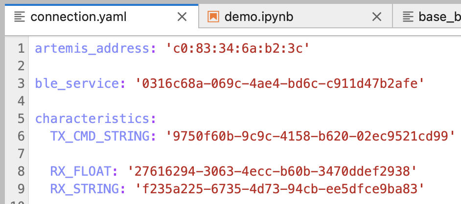
To connect to the Artemis the following lines were run in the Jupyter Notebook.

Several command types needed to be defined to complete the tasks outlined in the next section. Added commands include ECHO, GET_TIME_MILLIS, GET_TIME_MILLIS_LOOP, SEND_TIME_DATA, and GET_TEMP_READINGS.
Command types defined in Arduino IDE:
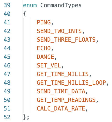
Command types defined in Jupyter Notebook:
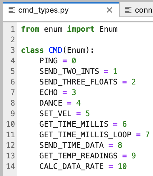
The first task was to send an ECHO command of a string value to the Artemis board and receive an augmented string on the host computer. This task tested the communication between the Artemis board and the computer.
The image below shows the Arduino IDE code.
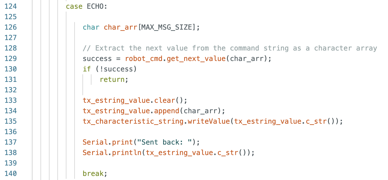
Jupyter Notebook code to send the ECHO command and receive the augmented string from the Artemis board:

The next task adds another command to the Jupyter Notebook for the Artemis board to reply with a string of the current time.
The image below shows the Arduino IDE code.

Jupyter Notebook code to send the GET_TIME_MILLIS command and receive the string with the current time:

A notification handler was created in the Python Jupyter Notebook to receive a string value from the Artemis board. The GET_TIME_MILLIS command was used to get the time after starting the notification handler.
The image below is the notification handler and the GET_TIME_MILLIS command in the Jupyter Notebook.
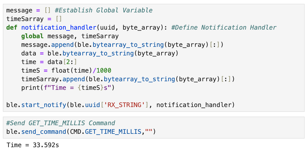
A loop was implemented to get the current time in milliseconds from the Artemis board and send the information to the computer. The time information is received and processed by the notification handler.
To find the data transfer rate the length of the data was computed by assembling the individual outputs into an array in the Jupyter Notebook. The number of strings in each element of the array is 9, and the number of elements in the array is 748. The time difference of the final (40.428s) and starting time (35.434s) was found to be 4.994 seconds. The data transfer rate is (748*9)bytes/4.994seconds = 1348.018 bytes/second
The image below shows the Arduino IDE code for case GET_TIME_MILLIS_LOOP.
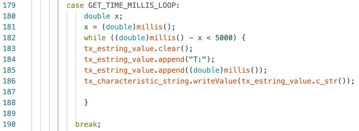
The image below shows the Jupyter Notebook command and some of the time outputs.
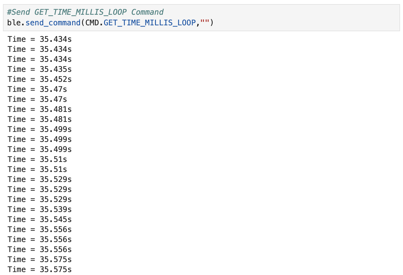
The following statements in Jupyter Notebook printed the timeSarray and the length of the array that was used to compute the data transfer rate.

The video below shows all of the time outputs.
A globally defined array to store time stamps was implemented. Inside of the for loop each time stamp is put inside of the “timearray”. The data is then sent as an array to the computer using Jupyter Notebook.
To find the data transfer rate the length of the data was computed by assembling the individual outputs into an array in the Jupyter Notebook. The number of strings in each element of the array is 9, and the number of elements in the array is 2748. The time difference of the final (49.730s) and starting time (49.685s) was found to be 0.045 seconds. The data transfer rate is (2748*9)bytes/0.045seconds = 549600 bytes/second
The image below shows the Arduino IDE code.
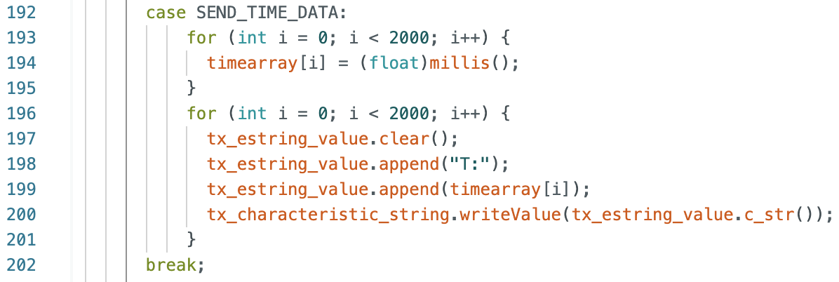
The image below shows the Jupyter Notebook command and some of the time outputs in the array.
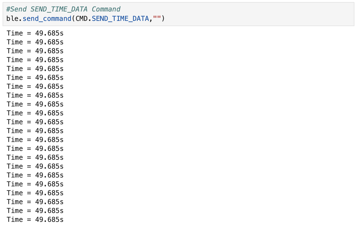
The following statements in Jupyter Notebook printed the timeSarray and the length of the array that was used to compute the data transfer rate.

The video below shows all of the times in the array.
A second array was added to store temperature readings from the Artemis board. The temperature array is the same size as the time array. The time and temperature readings were taken at the same time. The data is sent as an array to the computer using Jupyter Notebook.
The image below shows the Arduino IDE code.
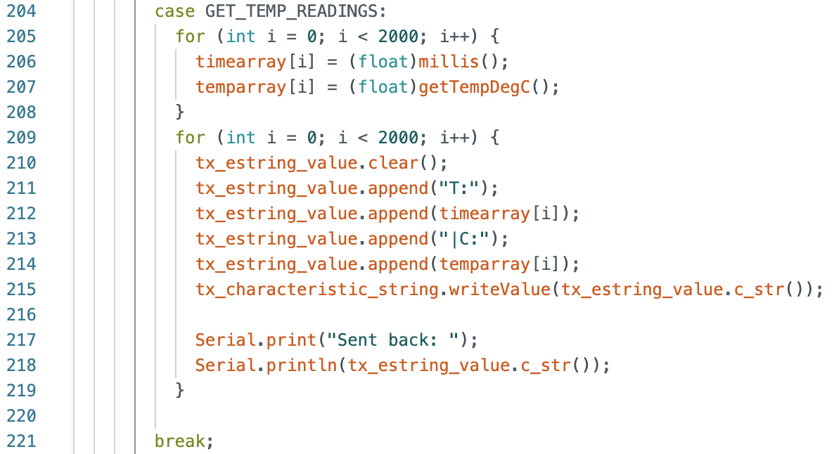
The image below shows the Jupyter Notebook command and some of the time and temperature outputs in the array.
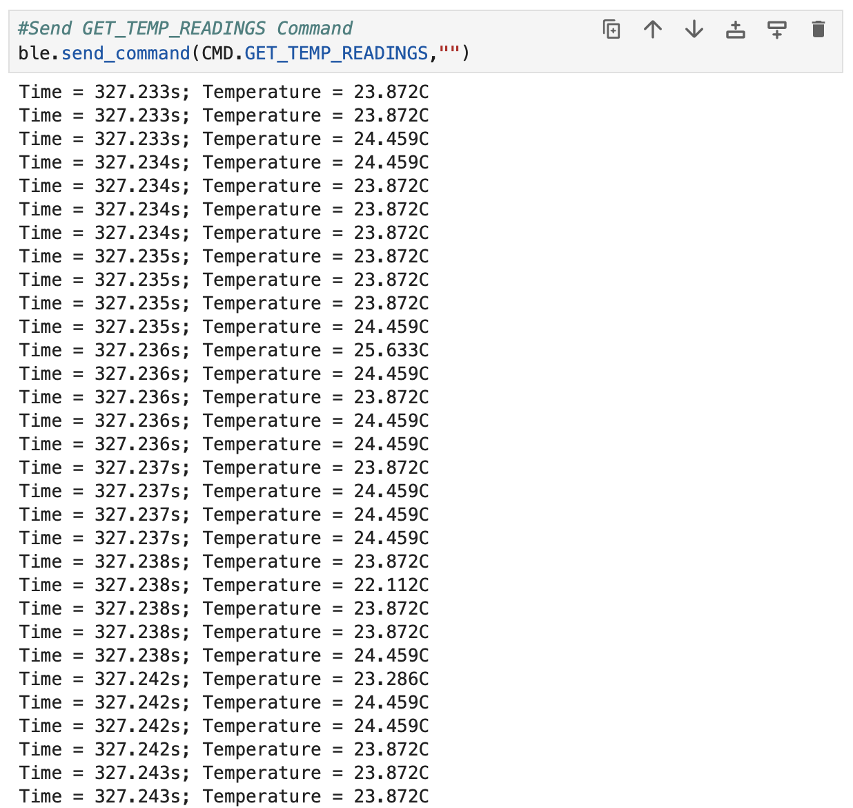
The video below shows all of the times and temperatures in the array.
The method used in Task 4 involved sending the current time from the Artemis board to the computer. Each time was sent as an individual piece of data. The method used in Task 5 involved creating an array of times that was stored on the memory of the Artemis board and then sent to the computer to display the collected data.
The data transfer rate of the array method used in Task 5 (549600 bytes/second) is faster than the data transfer rate when sending individual pieces of data in Task 4 (1348.018 bytes/second).
An advantage of sending data individually as in Task 4 is that less memory on the Artemis board is being used, but the disadvantage is a slower data transfer rate. An advantage of sending data as an array as in Task 5 is that there is a faster data transfer rate, but a disadvantage is that more memory is being used on the Artemis to store the array.
The Artemis board has a maximum storage of 384 kB of RAM. If 16 bit values at 150 Hz were sampled every 5 seconds, 256 values would be stored before running out of memory on the Artemis board. The calculations can be found below.

I sent a message from the computer and received a reply from the Artemis board. The data rate for 5, 10, 20, 30, 40, 50, 60, 70, 80, 90, 100, 110, and 120 bytes was tested. The data rate for 5 bytes is 132.722 bytes/s and the data rate for 120 bytes is 2003.210 bytes/s. The plotted graph shows that as the number of bytes sent to the Artemis board increases, the data rate increases. Below are pictures of the Jupyter Notebook code, the graph, and the printed statements.
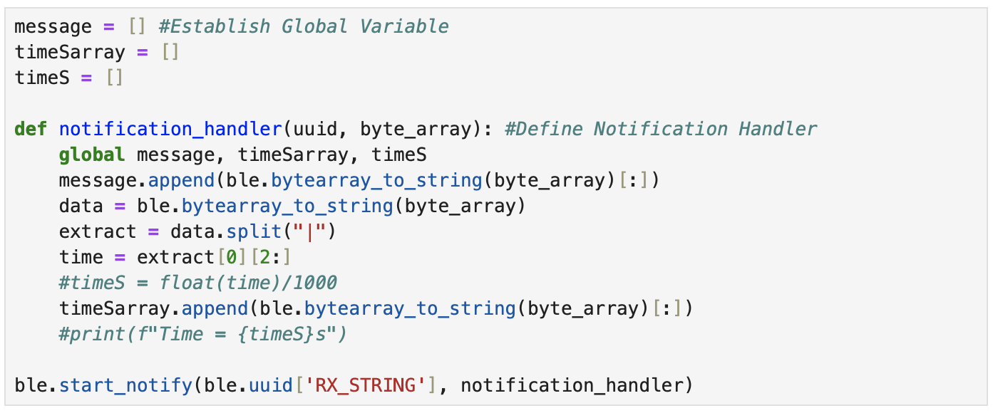
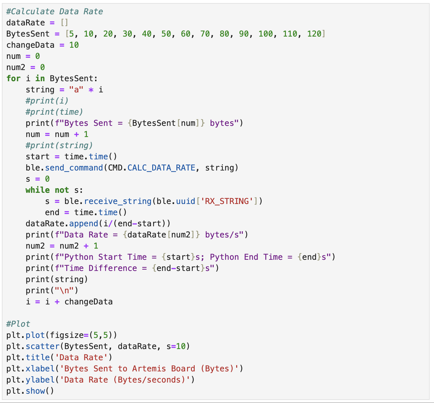
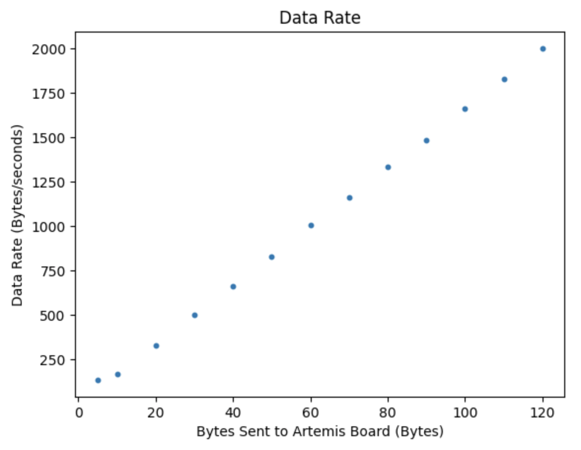
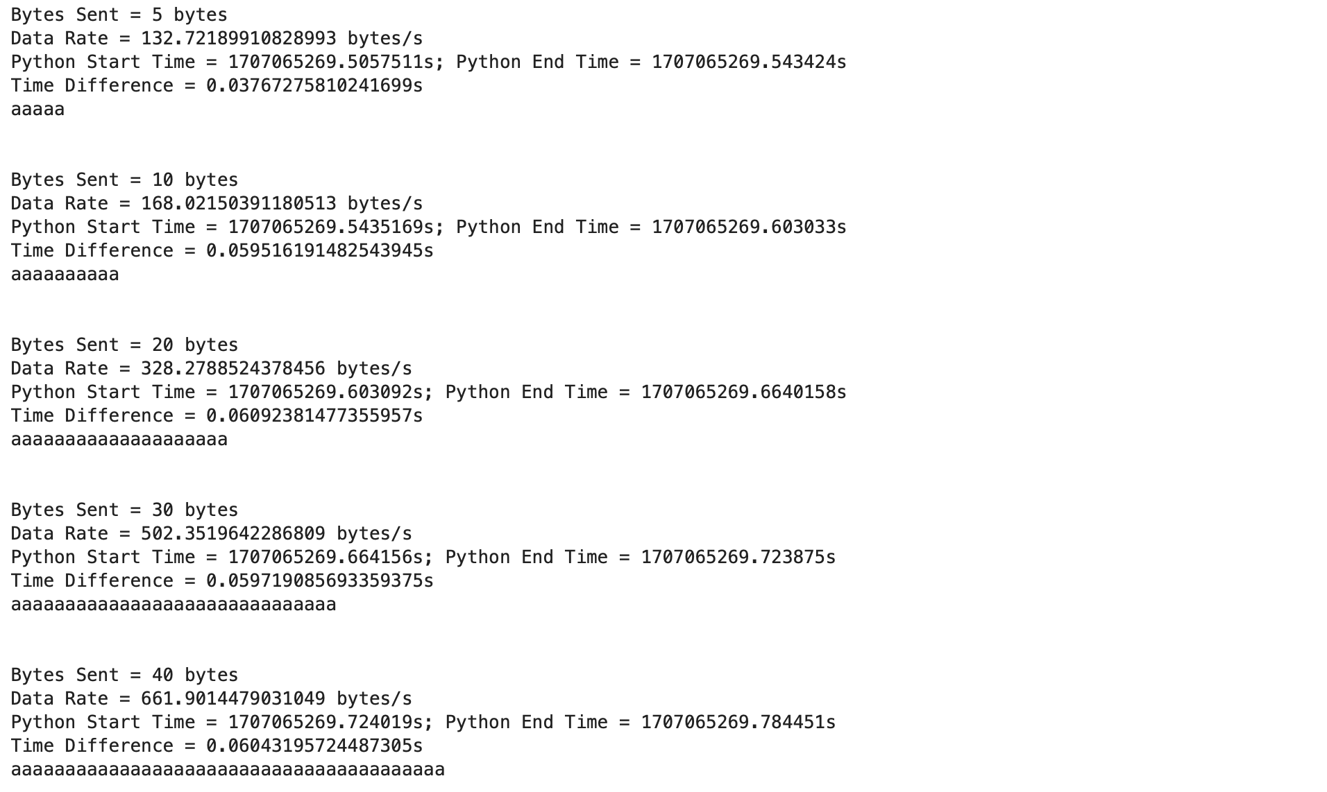
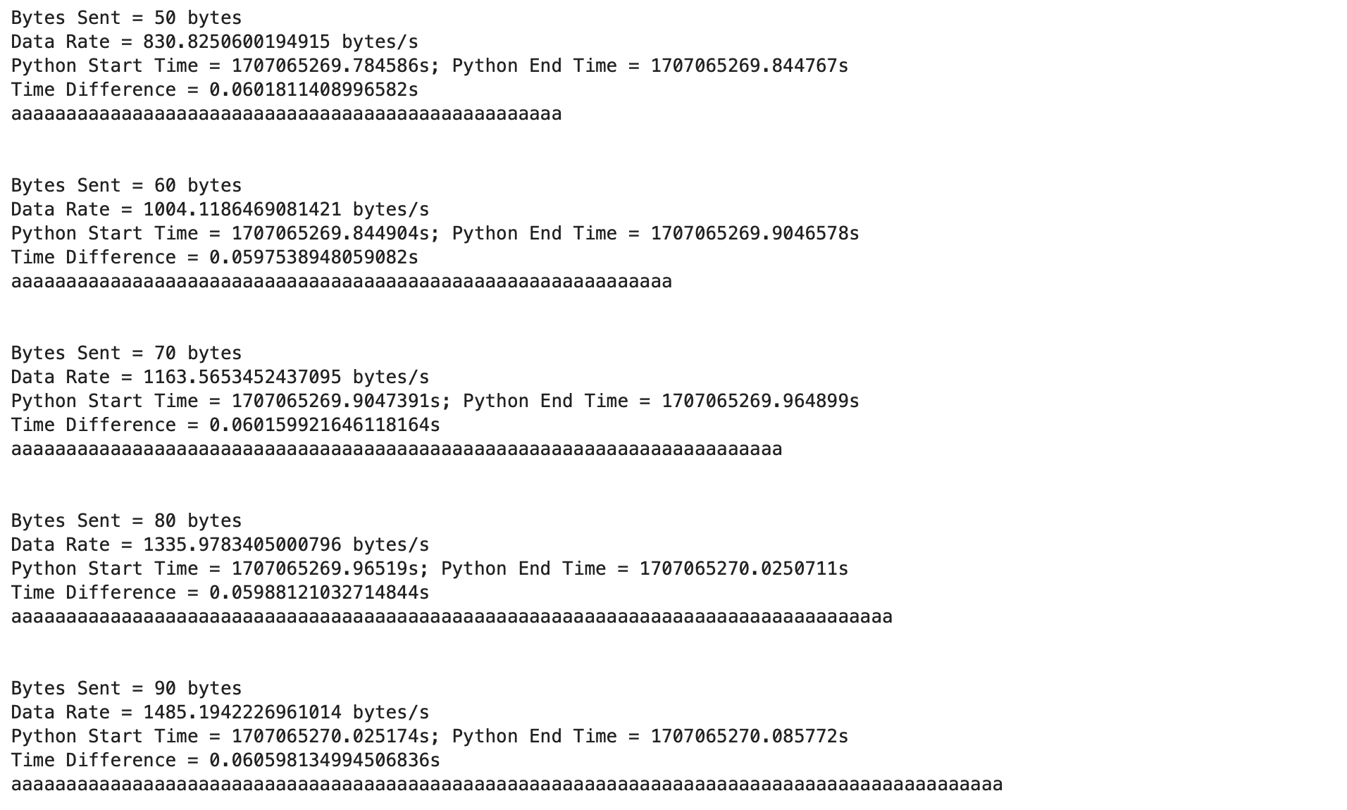
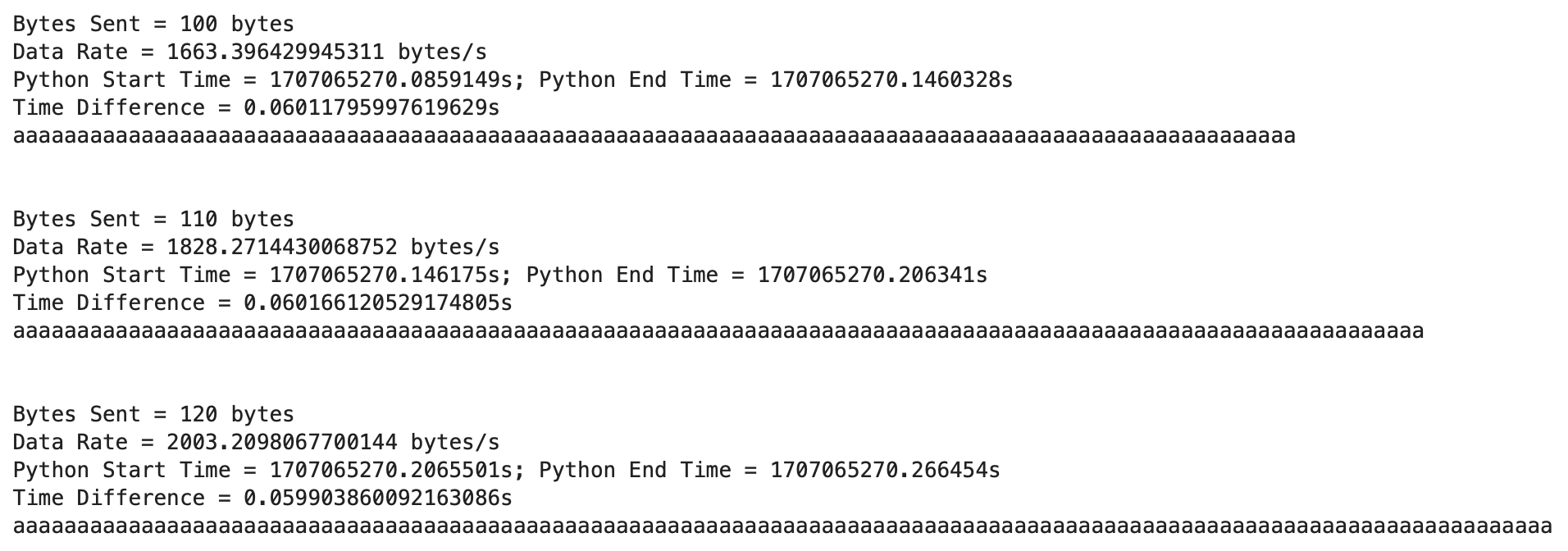
Additional graphs:
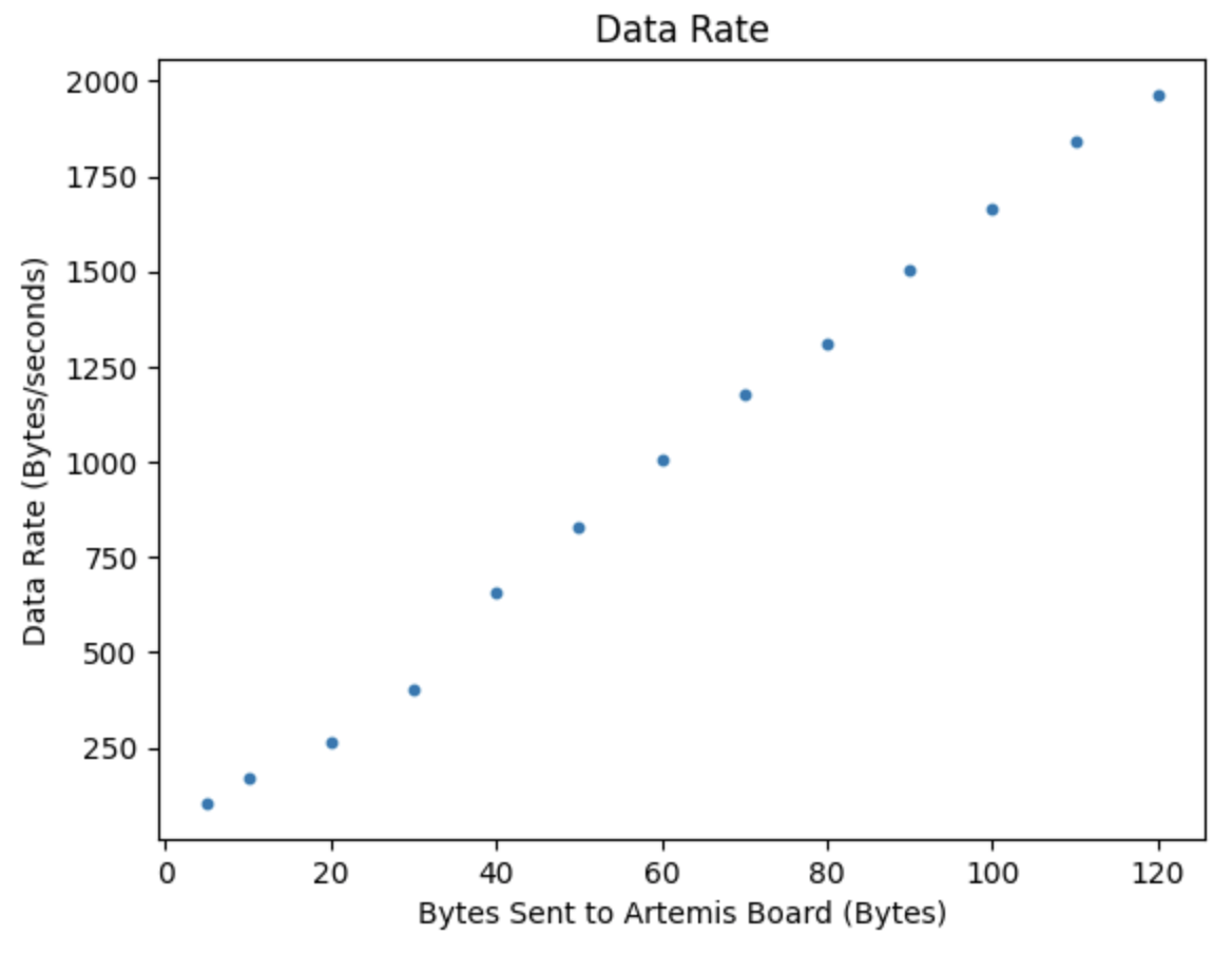
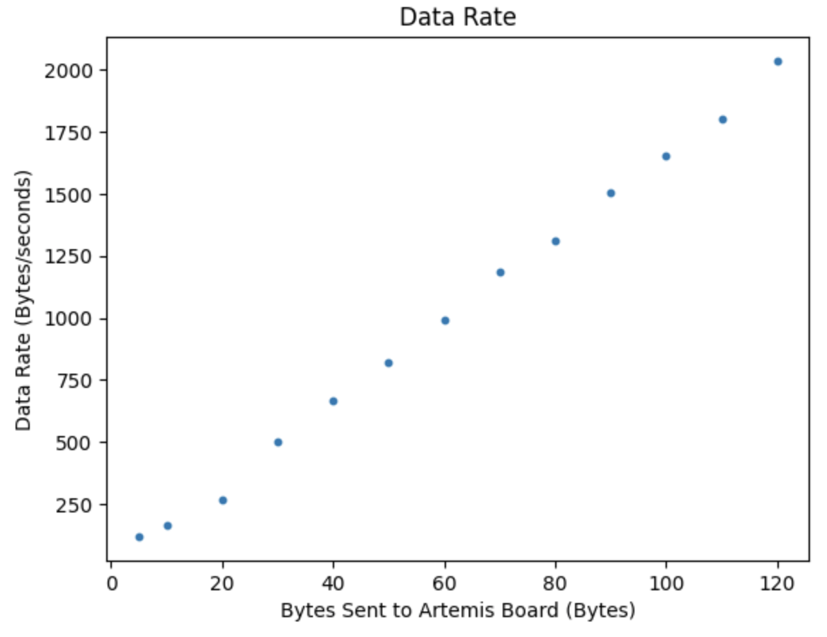
I tested the reliability of sending data at a higher rate from the robot to the computer. To determine the reliability of the data I ran the GET_TEMP_READINGS command and compared the outputs printed in the Jupyter Notebook and the Arduino IDE Serial Monitor.
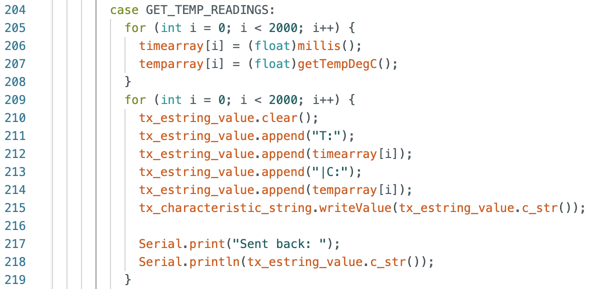
Outputs in the Jupyter Notebook (left) and the Arduino Serial Monitor (right):
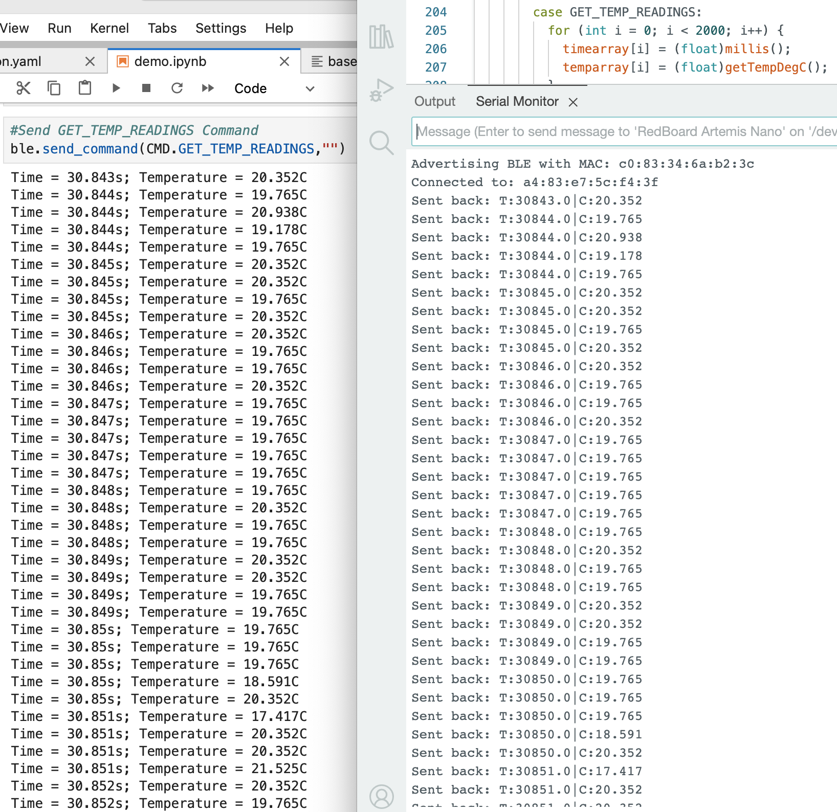
After looking at the outputs, the time and temperature readings on the computer are the same as the Artemis board and no data is missed. To confirm I copied and pasted the data from each window into Matlab variables titled time1 and temp1 for the Jupyter Notebook data, and time2 and temp2 for the Artemis data. I wrote a script to compare the corresponding time and temperature data and record how many data points are the same and how many are different. If there is a data point in the Jupyter Notebook that does not correspond to the Artemis board, or vice versa, an error message is displayed. The output variables in the workspace show that all data points are the same. The reliability is 100%.
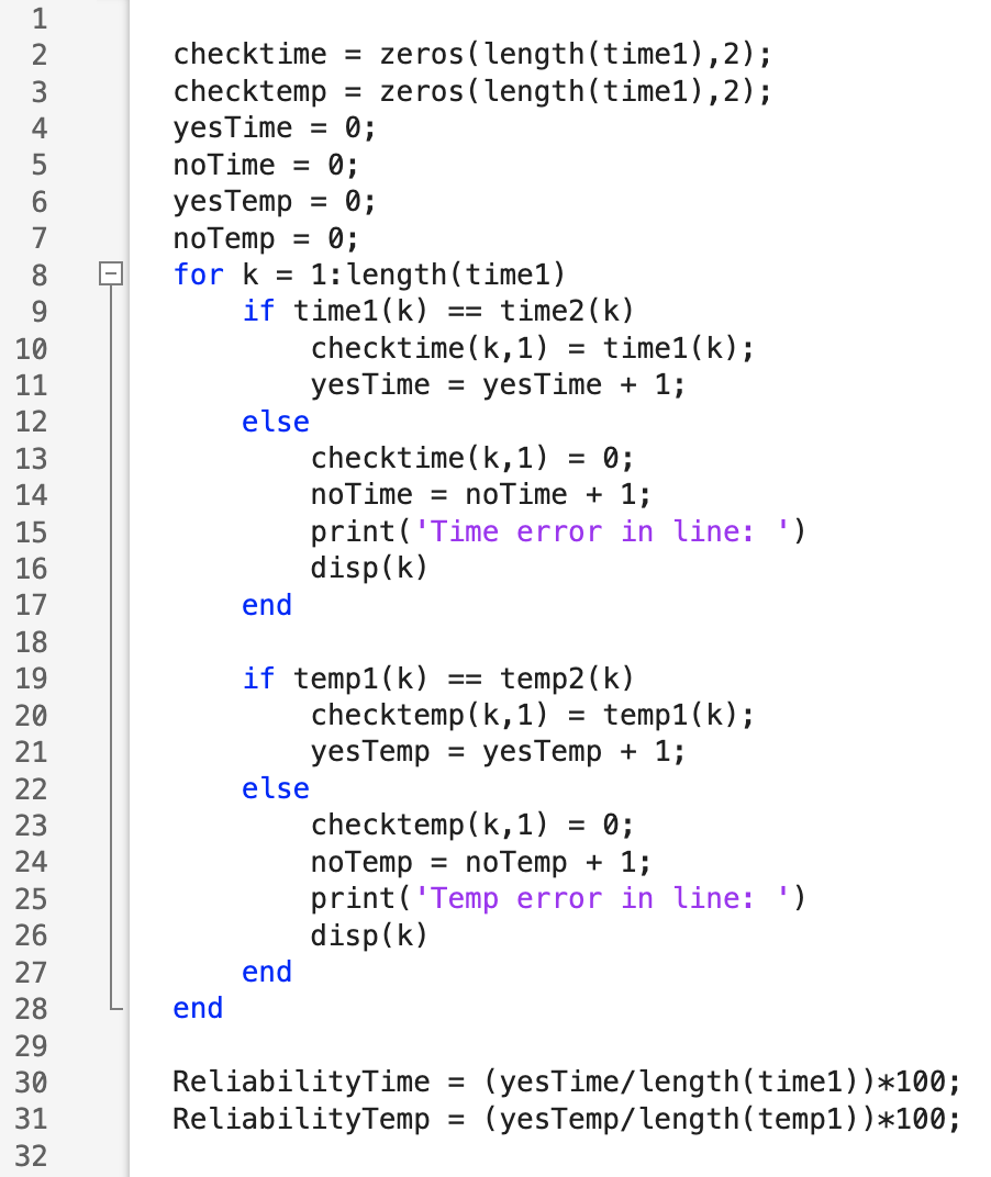
I learned how to use Bluetooth communication and UUIDs, between the Artemis board and computer. I did not experience any significant problems connecting to Bluetooth.
Thank you to all of the TAs that answered my questions. I referenced the past lab reports of Liam Kain, Rafael Gottlieb, Larry Lu, Julian Prieto, and Ignacio Romo.